Gather the outcomes that give each value and you get the probability mass function, one bar per value. Build it for the sum of two dice, a Galton board, a squared variable and flips until the first head, then set it beside a simulation.
Build the PMF of a discrete random variable by gathering the outcomes that give each value.
State the two properties of a PMF, never negative and summing to 1, and find P(X in a set) by adding bars.
Find the PMF of g(X) from the PMF of X by pooling the values that g sends to the same number.
Work with a PMF on infinitely many values, using a geometric series to check that it sums to 1.
Compute a PMF from scratch with Counter and Fraction and compare it with simulated relative frequencies.
In review. The maths and code on this page are checked by automated tests on every change, but an independent reader has not signed it off yet. Spot a mistake or a confusing step? Tell us.
The question
The sum of two dice can be anything from 2 to 12, but 7 turns up far more often than 2. A ball on a Galton board can land in any bin, yet it piles up in the middle. How do we describe, in one picture, how likely each value of a random variable is?
From the last lesson
1. What is a random variable?
Show answer
A function from the sample space \(\Omega\) to the real numbers: it gives each outcome \(\omega\) a number \(X(\omega)\).
2. For two dice and \({X = \text{sum}}\), what kind of object is \({\{X = 7\}}\), and how big is it?
Show answer
An event: the set of outcomes whose sum is 7. It holds 6 of the 36 outcomes.
Intuition
A random variable sorts the outcomes into piles, one pile for each value. The probability of a value is the probability of its pile. Draw one bar per value, as tall as that probability, and you have the probability mass function (PMF): the whole distribution of \(X\) in one picture.
M06.5.2-F1
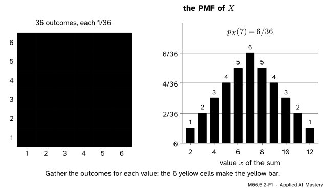
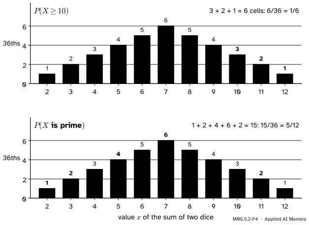
Each diagonal of the grid has one sum. Gather its cells and the count becomes the height of one bar: the PMF of the sum of two dice rises from \(1/36\) to \(6/36\) and falls back.
The grid’s diagonals do the counting. Sum 2 has one cell, \({(1, 1)}\); sum 3 has two; and so on up to sum 7 with six, after which the diagonals shorten again. Nothing is lost in this picture except the outcomes themselves: the PMF keeps how likely each value is and forgets which outcome gave it.
Build it up
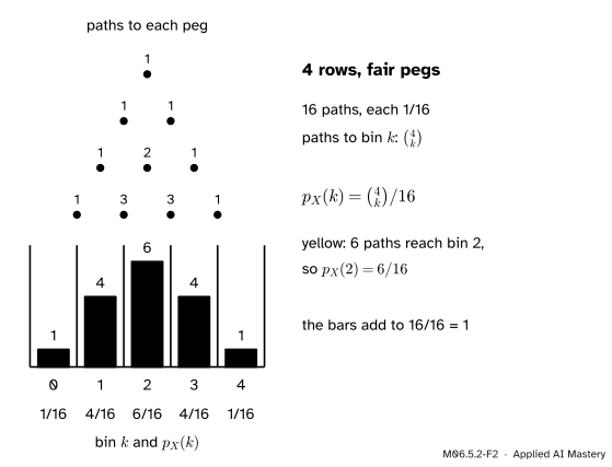
Step 1. A Galton board with 4 rows. Each of the \({2^4 = 16}\) paths is equally likely, \(1/16\) each, because every bounce is a fair left or right. Bin \(k\) collects the paths with \(k\) right bounces, and there are \(\binom{4}{k}\) of those: choose which \(k\) of the 4 bounces go right (lesson M06.2.3).
M06.5.2-F2
Pascal’s triangle on the pegs counts the paths. Each path has probability \(1/16\), so bin \(k\) gets \(\binom{4}{k}/16\).
So \({p_X(k) = \binom{4}{k}/16}\): the bars are 1, 4, 6, 4, 1 sixteenths. With \(n\) rows the same argument gives, for \({k = 0, 1, \dots, n}\),
\[
p_X(k) = \binom{n}{k} \frac{1}{2^n}.
\]
For 10 rows the middle bin gets \({\binom{10}{5}/1024} = {252/1024}\), about 0.246.
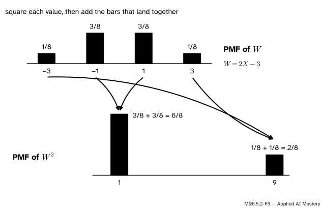
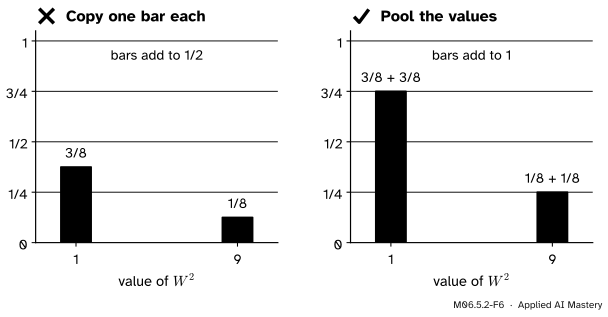
Step 2. A PMF for \(W^2\). Take the winnings of lesson M06.5.1, \({W = 2X - 3}\) for three flips, which is \({-3}\), \({-1}\), 1 or 3 with chances \(1/8\), \(3/8\), \(3/8\) and \(1/8\). Square it. The values \(1\) and \({-1}\) both square to 1, and \(3\) and \({-3}\) both square to 9. The event \({\{W^2 = 1\}}\) is \({\{W = -1\} \cup \{W = 1\}}\), two disjoint events, so their bars add.
M06.5.2-F3
Squaring sends two values of \(W\) to each value of \(W^2\), so the PMF of \(W^2\) adds two bars of \(W\) for each of its own.
Because \(W\) is symmetric about 0 (the bar at \(w\) matches the bar at \({-w}\)), each value of \(W^2\) gets exactly twice the bar of its positive root.
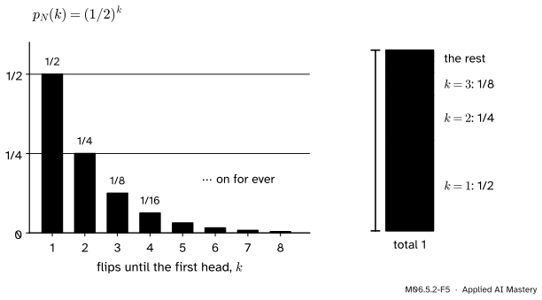
Step 3. Infinitely many values. Flip a fair coin until the first head and let \(N\) be the number of flips. \({N = k}\) means \({k - 1}\) tails and then a head, one particular string of \(k\) flips, so \({p_N(k) = (1/2)^k}\) for \({k = 1, 2, 3, \dots}\), with no largest value.
M06.5.2-F5
Each bar is half the one before, and laid end to end they fill a column of height 1: every piece takes half of what is left.
The formal statement
NoteDefinition: probability mass function
The probability mass function of a discrete random variable \(X\) is
\[
p_X(x) = \Prob(X = x)
\]
for every real number \(x\). It is 0 at every \(x\) that \(X\) never takes.
Two properties hold for every PMF, and both come from the fact that the events \({\{X = x\}}\) partition \(\Omega\) (lesson M06.5.1).
Never negative, never above 1.\({p_X(x) = \Prob(X = x)}\) is the probability of an event, so \({0 \leq p_X(x) \leq 1}\) by the axioms.
The bars add to 1. The events \({\{X = x\}}\), one for each value, are disjoint and together make up \(\Omega\). By additivity (over a list of events, if there are infinitely many values),
\[
\sum_{x} p_X(x) = \Prob(\Omega) = 1.
\]
Probabilities of sets of values. For any set \(A\) of numbers, the event \({\{X \in A\}}\) is the disjoint union of the events \({\{X = x\}}\) for \(x\) in \(A\), so
\[
\Prob(X \in A) = \sum_{x \in A} p_X(x).
\]
In the picture: shade the bars over \(A\) and add their heights.
The PMF of \(g(X)\). The event \({\{g(X) = y\}}\) is the union of the events \({\{X = x\}}\) over all \(x\) with \({g(x) = y}\). These are disjoint, so
So \(p_N\) is a genuine PMF, and sums of its bars give probabilities: for example \({\Prob(N \leq 3)} = {1/2 + 1/4 + 1/8} = {7/8}\).
Worked example
The sum of two dice. Find the PMF of \(X\), then \({\Prob(X \geq 10)}\) and \({\Prob(X \text{ is prime})}\).
The PMF. The cells on the diagonal for sum \(x\) number \({6 - \abs{x - 7}}\): 1 for \({x = 2}\), rising by one each step to 6 at \({x = 7}\), then falling back to 1 at 12. Each cell has probability \(1/36\), so for \({x = 2, 3, \dots, 12}\)
\[
p_X(x) = \frac{6 - \abs{x - 7}}{36}.
\]
Check. The counts add to 36, so the bars add to 1:
Once the PMF is built, neither question needs the grid again.
Code
From scratch: apply the random variable to every outcome, count the values with collections.Counter, and turn counts into exact fractions.
import itertoolsimport mathfrom collections import Counterfrom fractions import Fractionomega =list(itertools.product(range(1, 7), repeat=2))counts = Counter(a + b for a, b in omega) # value -> number of outcomespmf = {x: Fraction(counts[x], len(omega)) for x insorted(counts)}for x, p in pmf.items():print(x, p)print("total:", sum(pmf.values()))print("P(X >= 10) =", sum(p for x, p in pmf.items() if x >=10))print("P(X prime) =", sum(pmf[x] for x in (2, 3, 5, 7, 11)))
The PMF of a function of \(X\) pools bars. Here is \(W^2\) for three flips, and the Galton board with 4 and with 10 rows from math.comb.
flips = ["".join(s) for s in itertools.product("HT", repeat=3)]W = Counter(2* w.count("H") -3for w in flips)pmf_W = {w: Fraction(c, 8) for w, c insorted(W.items())}pmf_W2 = Counter()for w, p in pmf_W.items(): pmf_W2[w * w] += p # values that square alike pool their barsprint("PMF of W:", pmf_W)print("PMF of W squared:", dict(pmf_W2))galton4 = [Fraction(math.comb(4, k), 2**4) for k inrange(5)]print("Galton, 4 rows:", galton4)print("Galton, 10 rows, bin 5:", math.comb(10, 5) /2**10)
Now simulate. Roll two dice 100,000 times, find the distinct sums and how often each appears with numpy.unique(..., return_counts=True), and divide by the number of rolls to get relative frequencies.
import numpy as nprng = np.random.default_rng(7)sums = rng.integers(1, 7, size=100_000) + rng.integers(1, 7, size=100_000)values, freq = np.unique(sums, return_counts=True)shares = freq /len(sums)exact = np.array([float(pmf[x]) for x in values])for x, s, e inzip(values, shares, exact):print(f"{x:2d} simulated {s:.4f} exact {e:.4f}")print("largest gap:", np.max(np.abs(shares - exact)))
The simulated shares sit within a hundredth of the exact bars, but they are not equal to them, and a different seed gives slightly different shares. The PMF is what those shares settle towards.
Explore
M06.5-X1
Galton board
Drop one ball and follow its path: that is the outcome, and the lit bin is the value. Then drop a hundred at a time and watch the blue shares settle onto the exact PMF bars; try 1 row, then 10.
The middle bins fill fastest because more paths lead there, not because a ball prefers the middle: every path has the same probability. The tilt control, used again in M06.8.1, makes right bounces more or less likely than left ones.
Pitfalls
M06.5.2-F6
Wrong beside right. Copying one bar of \(W\) for each value of \(W^2\) loses half the probability; the total of 1/2 gives the mistake away.
“The PMF of \(W^2\) is the PMF of \(W\) at the square root.”
Both \({-1}\) and 1 square to 1, so \({\{W^2 = 1\}}\) contains both events. Taking only \({p_W(1) = 3/8}\) gives bars that add to \(1/2\). Pooling gives \(3/4\) and \(1/4\), which add to 1. Checking that the bars add to 1 catches this mistake every time.
“The bar heights of a histogram are the PMF.”
A histogram of 100,000 simulated rolls shows relative frequencies, and they wobble: another seed gives other heights. The PMF is exact, the limit those frequencies settle towards. A histogram of raw counts is further off still, since its bars add to the number of rolls, not to 1.
“Every value of \(X\) is equally likely, because every outcome is.”
Equally likely outcomes do not make equally likely values: the sum 7 has six outcomes and the sum 2 has one. The 11 sums are not each \(1/11\) (lesson M06.2.1). Gather the outcomes first; the PMF inherits its shape from how many outcomes each value collects. A classifier’s predicted labels behave the same way: rare classes collect few examples.
Check yourself
Recall
1. Define the PMF of a discrete random variable \(X\).
Show answer
\({p_X(x) = \Prob(X = x)}\) for every real \(x\), the probability that \(X\) takes the value \(x\); it is 0 at values \(X\) never takes.
2. What two properties does every PMF have?
Show answer
Every bar is between 0 and 1, and the bars add up to 1.
3. How do you find \({\Prob(X \in A)}\) from the PMF?
Show answer
Add the bars over the values in \(A\): \({\Prob(X \in A)} = {\sum_{x \in A} p_X(x)}\).
4. What is the PMF of the bin of a fair Galton board with \(n\) rows?
Show answer
\({p_X(k) = \binom{n}{k}/2^n}\) for \({k = 0, \dots, n}\): \(\binom{n}{k}\) paths end in bin \(k\), each with probability \({1/2^n}\).
5. Why do the bars of \({p_N(k) = (1/2)^k}\), \({k = 1, 2, \dots}\) add to 1?
Show answer
They form a geometric series with first term \(1/2\) and ratio \(1/2\), whose sum is \({(1/2)/(1 - 1/2) = 1}\).
Exercises
1.★ Let \(M\) be the larger of two dice. Show that \({p_M(m) = (2m - 1)/36}\) for \({m = 1, \dots, 6}\), check that the bars add to 1, and find \({\Prob(M \geq 5)}\).
Show solution
\({\{M = m\}}\) holds the outcomes where one die is \(m\) and the other is at most \(m\): the \(m\) cells \({(i, m)}\) with \({i \leq m}\) and the \(m\) cells \({(m, j)}\) with \({j \leq m}\), with the corner \({(m, m)}\) counted twice. That is \({m + m - 1 = 2m - 1}\) cells. The counts 1, 3, 5, 7, 9, 11 add to 36, so the bars add to 1. Then
2.★★ A fair Galton board has 5 rows. Write down its PMF and find the probability that a ball lands in bin 2 or bin 3.
Show solution
There are \({2^5 = 32}\) paths, and \(\binom{5}{k}\) end in bin \(k\): the counts are 1, 5, 10, 10, 5, 1, so \({p_X(k) = \binom{5}{k}/32}\). The bins are disjoint events, so
3.★★★ A random variable takes the values \({k = 1, 2, 3, \dots}\) with \({p(k) = c\,(1/3)^k}\). Find the constant \(c\) that makes this a PMF, then find \({\Prob(X \geq 3)}\) in two ways.
Show solution
The bars must add to 1. The geometric series with first term \(1/3\) and ratio \(1/3\) gives
Jeremy Orloff and Jonathan Bloom, Reading 4a: Discrete Random Variables, MIT OpenCourseWare 18.05, Spring 2022. Section 2.4 defines the pmf as \({p(a) = P(X = a)}\), notes that it is 0 at values \(X\) never takes, and tabulates the PMF of the maximum of two dice, 1/36, 3/36, …, 11/36, which is exercise 1 here.
NumPy documentation, numpy.unique: return_counts=True also returns “the number of times each unique item appears”, and the unique values come back sorted.