A random variable gives a number to every outcome of an experiment: the sum of two dice, the heads in three flips, the bin of a Galton board ball. See why statements such as X = 3 are events, and build random variables in Python as dictionaries.
Define a random variable as a function from the sample space to the real numbers, and give its value on a named outcome.
Write a statement about a random variable, such as X = 3 or X <= 3, as the set of outcomes it describes, and find its probability.
Build a new random variable g(X) from an old one, and an indicator from an event.
Store a random variable in Python as a dictionary from outcomes to values, and check an event’s probability by simulation.
In review. The maths and code on this page are checked by automated tests on every change, but an independent reader has not signed it off yet. Spot a mistake or a confusing step? Tell us.
The question
Roll two dice and the outcome is a pair, such as \({(3, 4)}\). Flip a coin three times and the outcome is a string, such as HTH. But the questions we ask are about numbers: what is the total, how many heads came up, which bin did the ball land in? How do we turn outcomes into numbers, so that “the total is 7” becomes something we can find a probability for?
Intuition
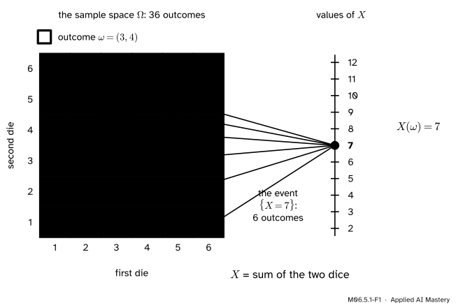
An experiment ends in one outcome \(\omega\) from its sample space \(\Omega\) (lesson M06.1.1). A random variable is a rule that reads the outcome and writes down a number. For two dice, the rule “add the two faces” turns the outcome \({(3, 4)}\) into the number 7. Every one of the 36 outcomes gets exactly one number, and many outcomes can get the same number.
M06.5.1-F1
The random variable \(X\) = sum of the two dice. Each outcome is sent to one number; the six yellow outcomes are all sent to 7, so “\({X = 7}\)” is a set of six outcomes.
Two things in the picture carry the whole lesson. First, \(X\) is a function: every cell holds exactly one number, its sum. The picture draws the arrows only for the six cells sent to 7, but every cell has one arrow, to its own sum. Nothing about it is random. The randomness is in which outcome happens; once it has happened, \(X\) simply reads off its number. Second, read the arrows backwards. Asking “is the total 7?” picks out the yellow cells, a subset of \(\Omega\). A subset of \(\Omega\) is an event (lesson M06.1.2), so it has a probability: 6 cells of 36, or \(1/6\).
Machine learning is full of random variables. Pick a test example at random: whether the model gets it right is a number, 1 or 0; the model’s loss on it is a number. The accuracy on a test set counts the 1s. Each is a function of which examples were drawn.
Build it up
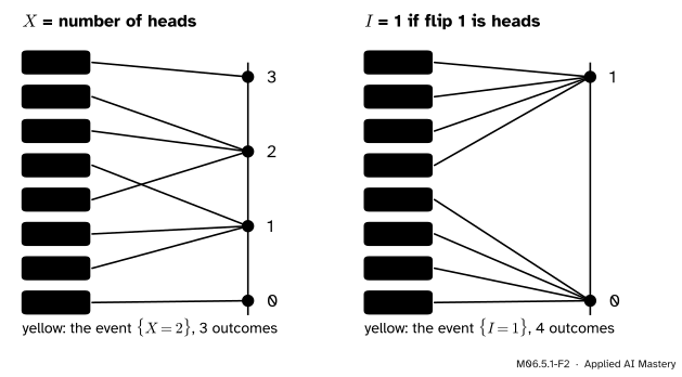
Step 1. One sample space, many random variables. Flip a fair coin three times. The sample space holds 8 equally likely strings, HHH to TTT. Let \(X\) be the number of heads. Then \({X(\text{HHT}) = 2}\) and \({X(\text{TTT}) = 0}\). On the same 8 outcomes we can define as many random variables as we like. Let \(I\) be 1 when the first flip is heads and 0 otherwise.
M06.5.1-F2
The same eight outcomes feed two different random variables. Each box sends exactly one line, and the yellow boxes are the event named underneath.
\(I\) is an indicator: a random variable that is 1 on an event and 0 off it. Here the event is “the first flip is heads”. Every event \(A\) has its indicator, written \(I_A\), and an indicator turns a yes-or-no question into a number that can be added up. The number of correct answers on a test set is a sum of indicators, one per example.
Step 2. Statements about \(X\) are events. Read \({\{X = 2\}}\) as “the set of outcomes on which \(X\) equals 2”. In the left panel it is \(\{\text{HHT}, \text{HTH}, \text{THH}\}\). In the same way, \({\{X \leq 1\}}\) is \(\{\text{HTT}, \text{THT}, \text{TTH}, \text{TTT}\}\). Since each of the 8 outcomes has probability \(1/8\),
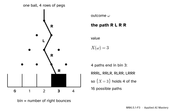
Step 3. The Galton board. A ball falls through 4 rows of pegs and bounces left or right at each. Its outcome is its path, a string such as RLRR, and there are \({2^4 = 16}\) paths. The bin it lands in is the number of right bounces: a random variable.
M06.5.1-F3
One ball’s outcome is its whole path; its value is a single number, the bin. Four different paths end in bin 3.
Step 4. A function of a random variable is a random variable. Suppose you win 1 for each head and lose 1 for each tail in three flips. Your winnings are heads minus tails, \({W = X - (3 - X) = 2X - 3}\). On HHT, \({W = 2 \cdot 2 - 3 = 1}\). \(W\) takes the values \({-3}\), \({-1}\), 1 and 3, and it is again a function of the outcome: first find \(X(\omega)\), then apply \({g(x) = 2x - 3}\).
The formal statement
NoteDefinition: random variable
A random variable\(X\) on a sample space \(\Omega\) is a function
\[
X : \Omega \to \R
\]
that gives a real number \(X(\omega)\) to each outcome \(\omega\). It is discrete when the values it can take can be listed: finitely many, or as many as the whole numbers.
Upper-case \(X\) names the function; lower-case \(x\) names one value it might take. “\({X = x}\)” is short for an event:
Read the colon as “such that”. Inequalities work the same way, so \({\{X \leq x\}}\) is the set of outcomes whose value is at most \(x\). Because these are events, the rules of lesson M06.1.4 apply to them. For example, \({\{X \leq 1\}}\) and \({\{X \geq 2\}}\) are complements, so
\[
\Prob(X \geq 2) = 1 - \Prob(X \leq 1).
\]
Three facts follow straight from “a function gives each outcome exactly one value”.
The events \({\{X = x\}}\) for different values \(x\) are disjoint: one outcome cannot have two values.
Together they cover\(\Omega\): every outcome has some value. So they partition the sample space, and the next lesson builds on this.
If \(g\) is any function from \(\R\) to \(\R\), then \(g(X)\), the outcome’s value passed through \(g\), is again a random variable: \({g(X)(\omega)} = {g(X(\omega))}\).
The indicator of an event \(A\) is the random variable
Its two events are \({\{I_A = 1\} = A}\) and \({\{I_A = 0\} = A^c}\), so \({\Prob(I_A = 1) = \Prob(A)}\).
Go deeper: why every subset is allowed to be an event here
For a finite or listable sample space every subset of \(\Omega\) is an event, so \({\{X = x\}}\) always has a probability. For a continuous sample space, such as a spinner, the formal definition adds one condition: \({\{X \leq x\}}\) must be an event for every \(x\). Which sets may be events in such a space is the subject of measure theory (M11). Nothing in this module needs it.
Worked example
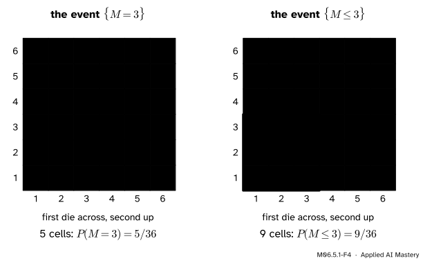
Two dice. Let \(M\) be the larger of the two numbers. Find \({\{M = 3\}}\) and \({\{M \leq 3\}}\) and their probabilities.
Values first.\(M\) gives each outcome the larger face: \({M(2, 5) = 5}\), \({M(4, 4) = 4}\), and \(M\) takes the values 1 to 6.
M06.5.1-F4
Each cell shows its value of \(M\). Left: the cells with value exactly 3 form an L. Right: the cells with value at most 3 fill the 3 by 3 corner.
The event \({\{M = 3\}}\). The larger number is 3 when one die shows 3 and the other shows 3 or less. Listing them:
That is 5 of 36 equally likely outcomes, so \({\Prob(M = 3) = 5/36}\).
The event \({\{M \leq 3\}}\). The larger number is at most 3 exactly when both dice are at most 3. The first die has 3 choices and the second has 3, so by the multiplication rule there are \({3 \times 3 = 9}\) outcomes, the corner square. So \({\Prob(M \leq 3)} = {9/36} = {1/4}\).
A check.\({\{M \leq 3\}}\) is the union of the disjoint events \({\{M = 1\}}\), \({\{M = 2\}}\) and \({\{M = 3\}}\), which have 1, 3 and 5 outcomes. And \({1 + 3 + 5 = 9}\). The same corner-square argument gives \({m^2}\) outcomes in \({\{M \leq m\}}\) for every \(m\) from 1 to 6, a fact lesson M06.5.3 uses.
Code
A random variable on a finite sample space is a lookup table, so a Python dictionary from outcomes to values stores it exactly. Events are sets, built by a comprehension.
import itertoolsfrom fractions import Fraction# The sample space: 36 ordered pairs (first die, second die).omega =list(itertools.product(range(1, 7), repeat=2))# Two random variables, each a dictionary from outcome to value.X = {w: w[0] + w[1] for w in omega} # the sumM = {w: max(w) for w in omega} # the larger facedef prob(event):"""Probability of a set of outcomes, all 36 equally likely."""return Fraction(len(event), len(omega))sum_is_7 = {w for w in omega if X[w] ==7}m_is_3 = {w for w in omega if M[w] ==3}m_at_most_3 = {w for w in omega if M[w] <=3}print("X(3, 4) =", X[(3, 4)], " P(X = 7) =", prob(sum_is_7))print("{M = 3} =", sorted(m_is_3), " P =", prob(m_is_3))print("P(M <= 3) =", prob(m_at_most_3))
The same pattern handles three flips, an indicator and a function of a random variable. The function \(g\) is applied to the value, so \(W\) is built from \(X\) without looking at the outcome again.
flips = ["".join(s) for s in itertools.product("HT", repeat=3)]heads = {w: w.count("H") for w in flips}first_is_head = {w: 1if w[0] =="H"else0for w in flips} # an indicatordef g(x):return2* x -3W = {w: g(heads[w]) for w in flips} # heads minus tailsdef p3(event):return Fraction(len(event), len(flips))print("P(X = 2) =", p3({w for w in flips if heads[w] ==2}))print("P(X <= 1) =", p3({w for w in flips if heads[w] <=1}))print("P(I = 1) =", p3({w for w in flips if first_is_head[w] ==1}))print("W(HHT) =", W["HHT"], " values of W:", sorted(set(W.values())))
Last, a simulation. Roll two dice 100,000 times with a seeded generator, apply \(M\) to each roll, and count how often \({M \leq 3}\). The share should be close to \(1/4\).
import numpy as nprng = np.random.default_rng(2026)rolls = rng.integers(1, 7, size=(100_000, 2)) # each row is one outcomem_values = rolls.max(axis=1) # M applied to every outcome at onceshare = np.mean(m_values <=3)print("share with M <= 3:", share)
share with M <= 3: 0.25116
The share lands within a hundredth of \(1/4\). The exact digits depend on the seed, which is why the check allows a small tolerance rather than an exact match.
Explore
This module’s interactive, the Galton board, lives in lesson M06.5.2. Drop one ball at a time and watch it: the path it draws is the outcome \(\omega\), and the bin it lights is the value \(X(\omega)\).
Pitfalls
M06.5.1-F5
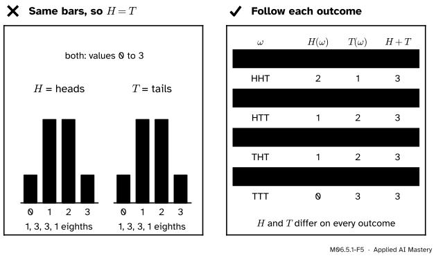
Wrong beside right. Heads and tails in three flips have identical bar charts, yet on every single outcome they differ.
“Heads and tails have the same chances, so they are the same random variable.”
Same chances is not same function. Let \(H\) count heads and \(T\) count tails in three flips. Both take 0, 1, 2, 3 with chances \(1/8\), \(3/8\), \(3/8\), \(1/8\). But \({H + T = 3}\) on every outcome, so \({H(\omega) = T(\omega)}\) would need \({H(\omega) = 1.5}\), which never happens: \({\Prob(H = T) = 0}\). Two random variables are equal only when they agree outcome by outcome. When they merely have the same chances, they are said to have the same distribution, the subject of the next lesson.
“A random variable is a random number.”
It is a fixed rule, a function. The randomness lives in which outcome happens. That is why \({X(3, 4) = 7}\) is a plain fact and not a probability, and why two random variables on the same \(\Omega\) can be added outcome by outcome: \({(X + Y)(\omega)} = {X(\omega) + Y(\omega)}\).
“\({\{X = 7\}}\) is the number 7.”
\({\{X = 7\}}\) is a set of outcomes; 7 is a value. Mixing them up leads to nonsense such as “\(\Prob(7)\)”. Write \({\Prob(X = 7)}\), the probability of the event, which is \(6/36\) for the sum of two dice.
Check yourself
Recall
1. What is a random variable, in one sentence?
Show answer
A function from the sample space \(\Omega\) to the real numbers: it gives a number \(X(\omega)\) to every outcome \(\omega\).
2. For three flips with \(X\) the number of heads, which outcomes make up \({\{X = 2\}}\)?
Show answer
HHT, HTH and THH, so \({\Prob(X = 2) = 3/8}\).
3. What is the indicator of an event \(A\), and what is \({\Prob(I_A = 1)}\)?
Show answer
The random variable that is 1 on outcomes in \(A\) and 0 elsewhere. \({\Prob(I_A = 1) = \Prob(A)}\).
4. Why are the events \({\{X = x\}}\), for different values \(x\), disjoint?
Show answer
A function gives each outcome exactly one value, so no outcome can lie in two of them.
5. On a Galton board, what is the outcome and what is the random variable?
Show answer
The outcome is the ball’s whole path of left and right bounces. The random variable is its bin, the number of right bounces.
Exercises
1.★ Two dice. Let \({D} = {\text{first} - \text{second}}\). Which values can \(D\) take? List the outcomes in \({\{D = 2\}}\) and find \({\Prob(D = 2)}\).
Show solution
The difference runs from \({1 - 6 = -5}\) to \({6 - 1 = 5}\), so \(D\) takes the 11 whole numbers from \({-5}\) to 5. The first die must be 2 more than the second:
2.★★ Three flips. Let \(Y\) be 1 if all three flips are the same and 0 otherwise. Write \(Y\) as a function of \(X\), the number of heads, write \({\{Y = 1\}}\) in terms of \(X\), and find \({\Prob(Y = 1)}\).
Show solution
All three flips are the same exactly when there are 0 heads or 3 heads, so \({Y = g(X)}\) with \({g(0) = g(3) = 1}\) and \({g(1) = g(2) = 0}\). Then \(Y\) is the indicator of that event, and
The two events are disjoint, so \({\Prob(Y = 1)} = {1/8 + 1/8} = {1/4}\).
3.★★★ A Galton board has \(n\) rows. Let \(X\) be the bin (right bounces) and \(L\) the number of left bounces. Explain why \({X + L = n}\) on every outcome. Describe \({\{X = n\}}\) and find its probability. For \({n = 4}\), list \({\{X \geq 3\}}\) and find \({\Prob(X \geq 3)}\).
Show solution
Every bounce is either right or left, and there are \(n\) bounces, so on every path the two counts add to \(n\). The board has \(2^n\) equally likely paths. \({\{X = n\}}\) holds the one path that goes right every time, so \({\Prob(X = n) = 1/2^n}\). For \({n = 4}\), \({\{X \geq 3\}}\) is the union of the disjoint events \({\{X = 3\}}\), which holds RRRL, RRLR, RLRR and LRRR, and \({\{X = 4\}}\), which holds RRRR. That is 5 paths of 16, so \({\Prob(X \geq 3) = 5/16}\).
Summary card
A random variable is a function that gives every outcome a number.
M06.5.1-F1
Outcomes in, numbers out.
Definition.\({X : \Omega \to \R}\); \(X(\omega)\) is the value on outcome \(\omega\).
Statements are events.\({\{X = x\}}\) is the set of outcomes with value \(x\).
They partition \(\Omega\). Different values give disjoint events that cover \(\Omega\).
Functions of it.\(g(X)\) and the indicator \(I_A\) are random variables too.
Sources and next steps
Sources. Each was opened and checked against this lesson on 12 November 2026.
Jeremy Orloff and Jonathan Bloom, Reading 4a: Discrete Random Variables, MIT OpenCourseWare 18.05, Spring 2022. Section 2.2 defines a discrete random variable as a function from \(\Omega\) to the real numbers on the two-dice sample space; Section 2.3 reads \({X = a}\) as the event of all outcomes with \({X(\omega) = a}\); Section 2.4 uses the maximum of two dice, as the worked example here does.
Chris Piech, Random Variables, Probability for Computer Scientists. Lower case for values that are not random, and “the scenario where a random variable takes on a particular value (or range of values) is an event”.