Write Bayes’ rule in odds and it becomes one multiplication: posterior odds equal prior odds times the likelihood ratio. Use it to update on a second positive test, then take logarithms and watch evidence add up, the way logistic regression does.
Convert between a probability and odds in both directions.
Derive the odds form of Bayes’ rule, posterior odds equal the likelihood ratio times the prior odds, and compute a likelihood ratio.
Update twice on evidence that is conditionally independent given the hypothesis, using the first posterior as the second prior.
Turn the products into sums with logarithms, and explain why logistic regression models the log-odds as a line.
In review. The maths and code on this page are checked by automated tests on every change, but an independent reader has not signed it off yet. Spot a mistake or a confusing step? Tell us.
The question
Your test for the course’s condition came back positive, so your chance of having it is now 1 in 12. The doctor orders a second, independent test, and it is positive too. What is the chance now? There is a way to answer in your head: one multiplication per test.
From the last lesson
1. On the grid of 1,000 people for the course’s test, how many true positives and how many false positives are there?
Show answer
9 true positives (90% of the 10 with the condition) and 99 false positives (10% of the 990 without it).
2. For the course’s test, what is the posterior after a positive result at base rates of 10% and 50%?
Show answer
\({1/2}\) at 10% and \({9/10}\) at 50%, from \({9\pi / (1 + 8\pi)}\).
Intuition
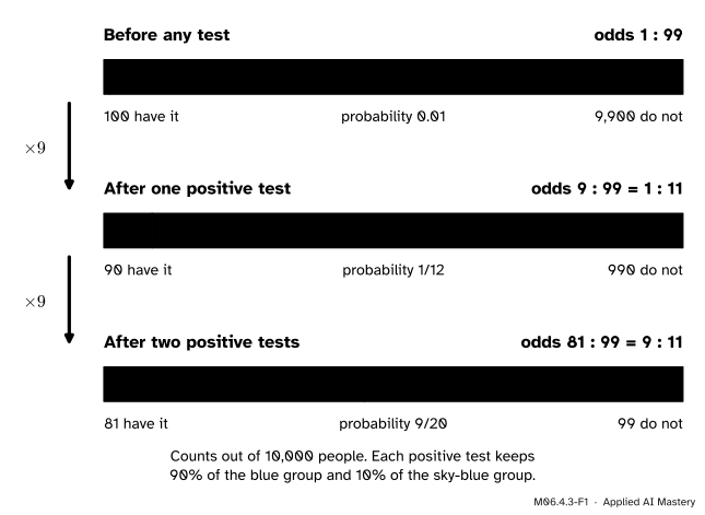
Picture 10,000 people. At a base rate of 1%, 100 have the condition and 9,900 do not: for every person with it there are 99 without. That ratio, 1 to 99, is the odds of having the condition.
A positive test keeps 90% of the people with the condition and 10% of the people without it. So it keeps 90 of the 100 and 990 of the 9,900. The ratio is now 90 to 990, which is 1 to 11. A second independent test does the same again: 81 of the 90 and 99 of the 990, so 81 to 99, which is 9 to 11.
M06.4.3-F1
Each positive test multiplies the odds by 9, because it keeps 90% of one group and 10% of the other, and \({0.9 / 0.1 = 9}\).
That factor of 9 is the whole story of the test. It does not depend on where you start: it turns 1 to 99 into 1 to 11, and 1 to 11 into 9 to 11. After two positive tests the probability is \({9/(9 + 11) = 9/20}\), nearly a half.
Build it up
Step 1. Odds are a second way to write a probability. The odds of an event \(A\) are
“Odds of 1 to 11” means \({O = 1/11}\): one person with the condition for every 11 without. To go back, solve \({o = p/(1 - p)}\) for \(p\): multiply out to get \({o - op = p}\), so \({o = p(1 + o)}\) and
\[
p = \frac{o}{1 + o} .
\]
A probability of \({1/12}\) is odds of \({(1/12) / (11/12) = 1/11}\), and odds of \({9/11}\) are a probability of \({(9/11)/(20/11) = 9/20}\). Probabilities run from 0 to 1; odds run from 0 to infinity, with even odds, 1, at probability one half.
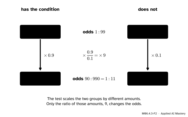
Step 2. The test scales each group by its own likelihood.
M06.4.3-F2
The people with the condition are multiplied by \({\Prob(+ \mid D) = 0.9}\), the others by \({\Prob(+ \mid D^c) = 0.1}\). The odds, a ratio of the two groups, are multiplied by the ratio \({0.9 / 0.1}\).
Step 3. Name the ratio. For a hypothesis \(H\) and evidence \(E\), the likelihood ratio is
For a positive result on the course’s test, \({\Lambda = 0.9/0.1 = 9}\). For a negative result it is \({\Prob(- \mid D) / \Prob(- \mid D^c)} = {0.1/0.9} = {1/9}\): a negative test divides the odds by 9. Evidence with \({\Lambda > 1}\) supports \(H\), evidence with \({\Lambda < 1}\) counts against it, and \({\Lambda = 1}\) is no evidence at all.
Step 4. A second test multiplies again. If the second test’s errors are fresh, it treats the two groups exactly as the first did, so it multiplies the odds by 9 once more.
The formal statement
NoteBayes’ rule in odds form
For a hypothesis \(H\) with \({0 < \Prob(H) < 1}\) and evidence \(E\) with \({\Prob(E \mid H^c) > 0}\),
In words: posterior odds equal the likelihood ratio times the prior odds.
Derivation. Write Bayes’ rule once for \(H\) and once for \(H^c\), and divide the first by the second. The evidence \(\Prob(E)\) appears in both and cancels:
The first fraction of the last line is \(\Lambda\) and the second is \(O(H)\). Notice what is missing: the odds form never needs the evidence \({\Prob(E)}\).
Two pieces of evidence. Let \(E_1\) and \(E_2\) be the two test results. They are conditionally independent given the hypothesis (M06.3.4) when, for \({H}\) and for \({H^c}\),
For two tests this says: among people with the condition, the second result has nothing to do with the first, and the same among people without it. Apply the odds form to the single event \({E_1 \cap E_2}\), and split its likelihood ratio with this rule:
Grouping it as \({\Lambda_2 \times (\Lambda_1 \times O(H))}\) is updating twice: the posterior odds after \(E_1\) become the prior odds for \(E_2\). It does not matter which test is read first.
Go deeper: why the first posterior is the right second prior
Updating on \(E_2\) after \(E_1\) means using Bayes’ rule with every probability conditioned on \(E_1\). The likelihood it needs is \({\Prob(E_2 \mid H \cap E_1)}\). By the definition of conditional probability, then the multiplication rule on top and bottom,
The last step uses conditional independence and cancels. So once \(H\) is known, \(E_1\) tells us nothing more about \(E_2\), and the second update uses the test’s ordinary likelihoods. The same holds with \(H^c\) in place of \(H\). Without conditional independence the second likelihood ratio must be worked out from \({\Prob(E_2 \mid H \cap E_1)}\) directly, which is the second pitfall below.
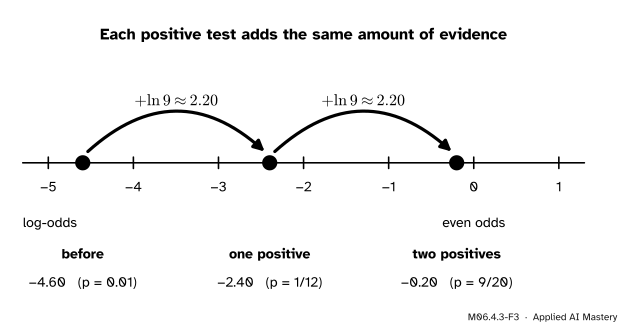
Logarithms turn products into sums. Take the natural logarithm of the two-test rule. The logarithm of a product is the sum of the logarithms (M01.4):
The log-odds start at the prior’s value, and each piece of evidence adds its own \({\ln \Lambda}\): a positive amount for evidence that supports \(H\), a negative amount for evidence against it.
M06.4.3-F3
On the log-odds line every positive test is the same step to the right, \({\ln 9 \approx 2.20}\). A negative test would be the same step to the left.
This is exactly the scale that logistic regression works on. Its score \({z = b + w_1 x_1 + \dots + w_d x_d}\) is the log-odds of the positive class (ML01.6.1): the bias \(b\) plays the part of the prior log-odds, and each feature adds its own amount of evidence. Lesson M06.4.4 shows that a naive Bayes classifier has the same shape.
Worked example
Two positive tests. Base rate 1%, likelihood ratio 9 for each positive result, and the two tests conditionally independent given the person’s state.
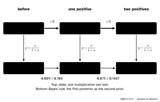
M06.4.3-F4
The same two updates done twice: by odds along the top, and by Bayes’ rule in probabilities along the bottom. Each column converts with \({p = o/(1 + o)}\).
By odds. The prior odds are \({0.01/0.99 = 1/99}\). After the first positive test they are \({9 \times 1/99 = 9/99 = 1/11}\). After the second they are \({9 \times 1/11 = 9/11}\). As a probability,
Both routes give \({9/20}\), but the odds route was two multiplications.
A positive, then a negative. The negative result has \({\Lambda = 1/9}\), so the odds go \({1/99 \to 1/11 \to 1/99}\): straight back to the base rate. The two results cancel exactly, because this test’s two likelihood ratios are 9 and \({1/9}\).
Code
First the conversions and the update, with exact fractions.
from fractions import Fraction as Frdef odds(p):return p / (1- p)def prob(o):return o / (1+ o)ratio_pos = Fr(9, 10) / Fr(1, 10) # likelihood ratio of a positive testratio_neg = Fr(1, 10) / Fr(9, 10) # likelihood ratio of a negative testo = odds(Fr(1, 100))history = [o]for ratio in (ratio_pos, ratio_pos): o = ratio * o # posterior odds = likelihood ratio x prior odds history.append(o)print("odds:", [str(x) for x in history], " probabilities:", [str(prob(x)) for x in history])print("positive then negative:", prob(ratio_neg * ratio_pos * odds(Fr(1, 100))))
A simulation with two tests that make their errors independently, given each person’s state:
import numpy as nprng = np.random.default_rng(seed=43)n =1_000_000has_it = rng.random(n) <0.01rate = np.where(has_it, 0.9, 0.1) # chance of a positive result, given the statetest1 = rng.random(n) < ratetest2 = rng.random(n) < rate # fresh random numbers: independent given the stateboth = test1 & test2print(f"{both.sum()} people test positive twice; a share {has_it[both].mean():.3f} have the condition")
17949 people test positive twice; a share 0.447 have the condition
On the log-odds scale the updates are additions. scipy.special.logit is the log-odds, \({\ln(p/(1 - p))}\), and expit turns log-odds back into a probability.
The frequency grid of lesson M06.4.2 can show a second test. Set the base rate to 8.3%, about the \({1/12}\) left by the first positive result, keep the test at 90% and 10%, and read the posterior after a second positive: about 0.45, the \({9/20}\) of this lesson.
Pitfalls
M06.4.3-F5
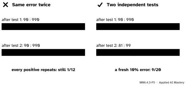
Wrong beside right. If the repeat makes the same mistake as the first test, everyone who was positive is positive again and the odds do not move. Only fresh errors multiply the odds again.
“Odds of 1 to 11 mean a probability of 1/11.”
Odds compare the two groups with each other, not one group with everyone. One person with the condition for every 11 without is 1 in 12 people: \({p} = {o/(1 + o)} = {(1/11)/(12/11)} = {1/12}\). For small probabilities the two are close, which is why the slip goes unnoticed; at even odds they are 1 and \({1/2}\).
“Two positive results always count as two pieces of evidence.”
Only when the results are conditionally independent given the person’s state. Suppose a test’s false positives come from a harmless substance in some people’s blood, and the repeat is run on the same blood. Everyone who was positive is positive again, so \({\Prob(+_2 \mid +_1, D^c) = 1}\) and \({\Prob(+_2 \mid +_1, D) = 1}\), the second likelihood ratio is 1, and the probability stays at \({1/12}\). Treating it as 9 claims \({9/20}\), more than five times too much. Naive Bayes makes this assumption about every pair of features, and is overconfident when features repeat each other (ML02.6).
“A positive test multiplies the probability by 9.”
It multiplies the odds by 9. The probability went from 0.01 to 0.083, about 8.3 times, and then from 0.083 to 0.45, about 5.4 times. A probability can never pass 1, while odds can grow without limit, which is why the multiplication belongs on the odds.
Check yourself
Recall
1. Convert a probability of \({1/12}\) to odds, and odds of \({9/11}\) to a probability.
Show answer
\({(1/12)/(11/12) = 1/11}\), that is 1 to 11. And \({(9/11)/(1 + 9/11) = 9/20}\).
2. State the odds form of Bayes’ rule.
Show answer
Posterior odds equal the likelihood ratio times the prior odds: \({O(H \mid E)} = {\Lambda \times O(H)}\), with \({\Lambda = \Prob(E \mid H) / \Prob(E \mid H^c)}\).
3. What are the likelihood ratios of a positive and of a negative result on the course’s test?
Show answer
\({0.9/0.1 = 9}\) for a positive result and \({0.1/0.9 = 1/9}\) for a negative result.
4. What must be true of two tests for the second to multiply the odds by its likelihood ratio again?
Show answer
They must be conditionally independent given the hypothesis: among people with the condition, and among people without it, the second result must not depend on the first.
5. On the log-odds scale, what does each piece of evidence do?
Show answer
It adds \({\ln \Lambda}\) to the log-odds: about 2.20 for a positive result on the course’s test, about \({-2.20}\) for a negative one.
Exercises
1.★ A third independent test is also positive. What is the probability of the condition now?
Show solution
The odds after two positives are \({9/11}\). A third positive multiplies them by 9: \({81/11}\). The probability is \({(81/11)/(1 + 81/11)} = {81/92} \approx {0.880}\).
2.★★ A screening test for a different condition has \({\Prob(+ \mid D) = 0.99}\) and \({\Prob(+ \mid D^c) = 0.02}\), and the base rate is 0.5%. Find the likelihood ratio of a positive result and the probability of the condition after one positive result.
Show solution
\({\Lambda = 0.99/0.02 = 49.5}\). The prior odds are \({0.005/0.995 = 1/199}\), so the posterior odds are \({49.5/199 \approx 0.249}\), about 1 to 4. The probability is \({49.5 / (199 + 49.5)} = {49.5/248.5} \approx {0.199}\). Bayes’ rule in probabilities agrees: \({0.00495 / (0.00495 + 0.0199)} = {0.00495/0.02485} \approx {0.199}\).
3.★★★ A person takes the course’s test \(n\) times, with independent errors given their state, and \(k\) results are positive. Show that the posterior log-odds are \({\ln(1/99) + (2k - n)\ln 9}\). How many positive results in a row are needed before the probability of the condition passes 0.99?
Show solution
Each positive adds \({\ln 9}\) and each of the \({n - k}\) negatives adds \({\ln(1/9) = -\ln 9}\), so the log-odds are \({\ln(1/99) + k\ln 9 - (n - k)\ln 9} = {\ln(1/99) + (2k - n)\ln 9}\). With \(k\) positives in a row the odds are \({9^k/99}\). A probability above 0.99 needs odds above \({0.99/0.01 = 99}\), so \({9^k > 99^2 = 9{,}801}\). Since \({9^4 = 6{,}561}\) and \({9^5 = 59{,}049}\), five positives are needed: four give \({p = 6{,}561/6{,}660 \approx 0.985}\) and five give \({59{,}049/59{,}148 \approx 0.998}\).
Summary card
Each piece of evidence multiplies the odds by its likelihood ratio.
Sources. Each was opened and checked against this lesson on 12 November 2026.
Jeremy Orloff and Jonathan Bloom, Reading 12b: Bayesian updating, odds, MIT OpenCourseWare 18.05, Spring 2022. Section 2 defines odds and gives the conversion formulas; Section 4 defines the Bayes factor (likelihood ratio) and derives posterior odds as the Bayes factor times the prior odds; Section 4.1 updates again under conditional independence; Section 5 adds log Bayes factors to the prior log-odds and notes the link to logistic regression.