Knowing how often spam contains ‘free’ is not the same as knowing how often a ‘free’ email is spam. Derive Bayes’ rule in two lines, name its four parts, and turn one conditional probability into the other on the inbox.
Derive Bayes’ rule in two lines from the definition of conditional probability.
Name the prior, the likelihood, the evidence and the posterior in a problem, and find the evidence with the law of total probability.
Compute a posterior by hand, on a probability tree read backwards, and with a short Python function.
Explain why P(A | B) and P(B | A) differ, and say when they are equal.
In review. The maths and code on this page are checked by automated tests on every change, but an independent reader has not signed it off yet. Spot a mistake or a confusing step? Tell us.
The question
A spam filter learns from emails that people have already labelled. Counting is easy in that direction: 60% of the spam contains the word ‘free’. But when a new email arrives with ‘free’ in it, the filter needs the opposite number: how likely is this email to be spam? The two numbers are not the same. How do you get from one to the other?
Intuition
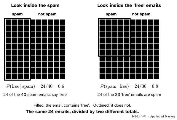
The course’s inbox has 100 emails: 40 are spam and 60 are not. The word ‘free’ appears in 24 of the spam emails and in 6 of the others. Lay the 100 emails out as a grid, with spam on the left, and fill in every email that contains ‘free’.
M06.4.1-F1
Two questions about the same grid. On the left we look inside the spam and ask how much of it says ‘free’. On the right we look inside the ‘free’ emails and ask how much of them is spam. The 24 emails that are both are the same in each picture; only the total they are divided by changes.
A conditional probability (M06.3.1) keeps only the outcomes in the condition and asks what share of them has the property. So the two questions use the same overlap and different totals:
\({\Prob(\text{free} \mid \text{spam}) = 24/40 = 0.6}\): the overlap divided by all the spam.
\({\Prob(\text{spam} \mid \text{free}) = 24/30 = 0.8}\): the overlap divided by all the ‘free’ emails.
Turning a conditional around means keeping the overlap and swapping the total. Bayes’ rule is that sentence written with probabilities instead of counts, so that it works when you do not have a grid to count, only the rates.
Build it up
Step 1. What we know runs forwards. A filter is trained on labelled email, so it knows how each kind of email behaves. In probabilities: \({\Prob(\text{spam}) = 0.4}\), \({\Prob(\text{free} \mid \text{spam}) = 0.6}\) and \({\Prob(\text{free} \mid \text{not spam}) = 0.1}\). Each of these starts from the kind of email and asks about the word.
Step 2. What we want runs backwards. The question starts from the word and asks about the kind: \({\Prob(\text{spam} \mid \text{free})}\).
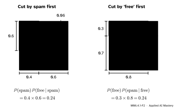
Step 3. The overlap can be built from either end. Picture the inbox as a unit square whose area is probability. Cut it first into a spam strip of width 0.4 and a not-spam strip of width 0.6, then cut each strip by its share of ‘free’. Or cut it first by ‘free’ and then by spam. Both routes end at the same piece of area.
M06.4.1-F2
One piece of area, measured two ways. On the left it is a width times a height, \({0.4 \times 0.6}\); on the right it is \({0.3 \times 0.8}\). Both give 0.24.
On the left, the multiplication rule of M06.3.2 gives the area as a product, and on the right the same rule with the roles swapped gives the same area as another product:
Step 4. Set the two equal and divide. The two products are equal, so dividing by \({\Prob(\text{free})}\) leaves the number we want. The only piece we were not given is \({\Prob(\text{free})}\), and the law of total probability (M06.3.3) supplies it: add the ‘free’ area in the spam strip to the ‘free’ area in the other strip, \({0.24 + 0.06 = 0.30}\). Then \({\Prob(\text{spam} \mid \text{free})} = {0.24 / 0.30} = {0.8}\), the same answer the grid gave.
The formal statement
NoteBayes’ rule
For events \(H\) and \(E\) with \({\Prob(H) > 0}\) and \({\Prob(E) > 0}\),
The same definition with \(H\) as the condition says \({\Prob(E \mid H) = \Prob(E \cap H) / \Prob(H)}\). Multiply both sides by \(\Prob(H)\), and use that \({E \cap H}\) and \({H \cap E}\) are the same event:
Put this into the numerator of the first line, and Bayes’ rule is proved. That is all: two uses of one definition.
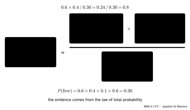
The letters stand for hypothesis and evidence, and each part has a name.
The prior\(\cparam{\Prob(H)}\) is how probable the hypothesis is before the evidence.
The likelihood\(\cdata{\Prob(E \mid H)}\) is how probable the evidence is if the hypothesis is true.
The evidence\(\Prob(E)\) is how probable the evidence is overall.
The posterior\(\cmodel{\Prob(H \mid E)}\) is how probable the hypothesis is after the evidence.
M06.4.1-F3
The four parts of Bayes’ rule, filled in with the inbox. The colours match the equation above.
The evidence by total probability. The hypothesis \(H\) and its complement \(H^c\) split \(\Omega\) into two pieces, so the law of total probability gives \(\Prob(E) = {\Prob(E \mid H)\,\Prob(H)} + {\Prob(E \mid H^c)\,\Prob(H^c)}\). Put that into the denominator and every term is something we usually know:
The numerator \(a\) is one of the two terms of the denominator. So the posterior is a share: the part of the evidence that comes through \(H\), out of all the evidence.
When are the two conditionals equal? Write the multiplication rule both ways, \({\Prob(H \mid E)\,\Prob(E)} = {\Prob(E \mid H)\,\Prob(H)}\), and divide (when \({\Prob(H \cap E) > 0}\)):
The two directions differ by the ratio of the two totals. They are equal exactly when \({\Prob(H) = \Prob(E)}\). In the inbox, \({0.8 / 0.6 = 0.4 / 0.3 = 4/3}\).
Go deeper: what a zero in Bayes' rule means
If \({\Prob(E) = 0}\) the rule says nothing, because \({\Prob(H \mid E)}\) is not defined: we cannot condition on something that cannot happen. If \({\Prob(E \mid H) = 0}\) and \({\Prob(E) > 0}\), the numerator is 0 and so is the posterior: evidence that is impossible under a hypothesis rules it out completely. Lesson M06.4.4 uses this when a die shows a 5 and the four-sided die drops out. The other zero is a warning. If \({\Prob(H) = 0}\), the posterior is 0 whatever the evidence, so a prior of exactly 0 can never be revised. That is why people who build models avoid priors of exactly 0 or 1.
Worked example
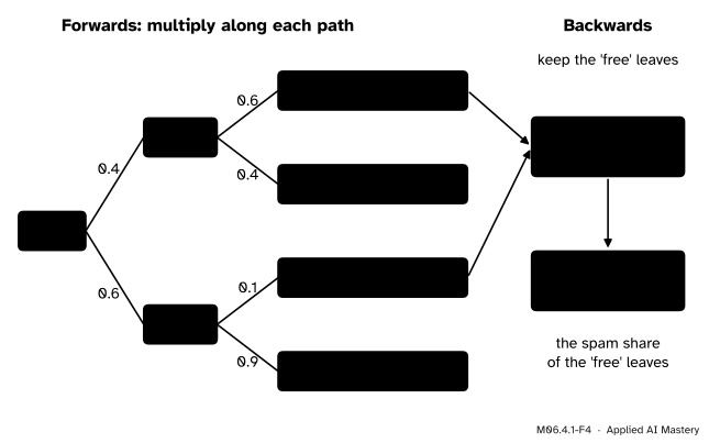
The inbox, by Bayes’ rule. We are given the prior \({\Prob(\text{spam}) = 0.4}\) and the two likelihoods \({\Prob(\text{free} \mid \text{spam}) = 0.6}\) and \({\Prob(\text{free} \mid \text{not spam}) = 0.1}\). Draw the tree forwards, multiply along each path, then read it backwards.
M06.4.1-F4
Forwards, the tree multiplies along each path. Backwards, it keeps the leaves where ‘free’ was seen, adds them to get the evidence, and asks what share of them came through spam.
The leaves are the four joint probabilities. Two of them have ‘free’:
Missing ‘free’ is weak evidence against spam, and the probability falls from 0.4 to about 0.23. The two posteriors average back to the prior, weighted by how often each case happens: \({0.30 \times 0.8} + {0.70 \times 8/35} = 0.24 + 0.16 = 0.4\). Before you open an email, you cannot expect the evidence to push your belief up or down on average.
Code
First Bayes’ rule as a function of the three numbers we are given, with exact fractions.
from fractions import Fraction as Frdef bayes(prior, like_h, like_not_h):"""P(H | E) from the prior P(H) and the likelihoods P(E | H) and P(E | not H).""" evidence = like_h * prior + like_not_h * (1- prior) # law of total probabilityreturn like_h * prior / evidenceprior = Fr(4, 10)p_free = Fr(6, 10) * prior + Fr(1, 10) * (1- prior)print("P(free) =", p_free)print("P(spam | free) =", bayes(prior, Fr(6, 10), Fr(1, 10)))print("P(spam | no free) =", bayes(prior, Fr(4, 10), Fr(9, 10)))
The no-‘free’ case passes the likelihoods of not seeing the word, \({1 - 0.6}\) and \({1 - 0.1}\). Now the same answer by counting, the way the grid did it: list the 100 emails and keep the ones with ‘free’.
emails = ([("spam", True)] *24+ [("spam", False)] *16+ [("not spam", True)] *6+ [("not spam", False)] *54)with_free = [label for label, free in emails if free]print(len(with_free), "emails say 'free';", with_free.count("spam"), "of them are spam:", Fr(with_free.count("spam"), len(with_free)))
30 emails say 'free'; 24 of them are spam: 4/5
A simulation checks the rule without using it. Each simulated email is spam with probability 0.4, and then contains ‘free’ with probability 0.6 or 0.1. Among the simulated emails with ‘free’, we count the share that is spam.
import numpy as nprng = np.random.default_rng(seed=4)n =200_000spam = rng.random(n) <0.4free = np.where(spam, rng.random(n) <0.6, rng.random(n) <0.1)estimate = spam[free].mean()print(f"{free.sum()} simulated emails say 'free'; the share that is spam is {estimate:.3f}")
59559 simulated emails say 'free'; the share that is spam is 0.799
The share settles close to 0.8; another seed would give a slightly different third decimal. Finally, pandas builds the whole table of conditional shares at once. With normalize="columns" each column is divided by its own total, so the column for ‘free’ holds \({\Prob(\text{spam} \mid \text{free})}\).
import pandas as pdtable = pd.crosstab(pd.Series(spam, name="spam"), pd.Series(free, name="free"), normalize="columns")print(table.round(3))
This module’s interactive, the frequency grid, is in the next lesson. It counts Bayes’ rule out on 1,000 people, as the grid above counted it on 100 emails.
Pitfalls
M06.4.1-F5
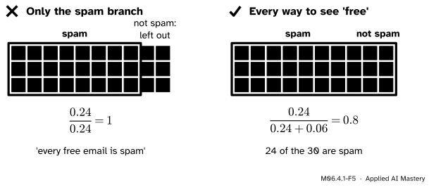
Wrong beside right. The evidence must count every way the evidence can happen. Leave out the not-spam branch and every ‘free’ email looks like spam.
“P(spam | free) and P(free | spam) are the same thing.”
They answer different questions and divide by different totals: 30 ‘free’ emails in one, 40 spam emails in the other. They differ by the factor \({\Prob(\text{spam}) / \Prob(\text{free})}\) and agree only when those two are equal. Mixing them up is so common that the next lesson gives it two names.
“The denominator is the likelihood of the hypothesis I care about.”
The evidence \(\Prob(E)\) counts every route to \(E\), through \(H\) and through \(H^c\). Dividing \({0.24}\) by \({0.24}\) alone gives 1, as in the left panel. The right denominator is \({0.24 + 0.06}\).
“The two likelihoods should add up to 1.”
\({\Prob(\text{free} \mid \text{spam}) = 0.6}\) and \({\Prob(\text{free} \mid \text{not spam}) = 0.1}\) add up to 0.7, and nothing is wrong. They are probabilities of the same event under two different conditions. What adds up to 1 is a pair with the same condition: the chances that a spam email does and does not say ‘free’ (0.6 and 0.4), or the two posteriors for an email that says ‘free’ (0.8 for spam and 0.2 for not spam). A naive Bayes classifier (ML02.6) stores one likelihood per word for each class, and these never need to add up to 1 across classes.
Check yourself
Recall
1. State Bayes’ rule and name its four parts.
Show answer
\({\Prob(H \mid E)} = {\Prob(E \mid H)\,\Prob(H) / \Prob(E)}\). \(\Prob(H)\) is the prior, \({\Prob(E \mid H)}\) the likelihood, \(\Prob(E)\) the evidence and \({\Prob(H \mid E)}\) the posterior.
2. Which single definition is used twice to derive Bayes’ rule?
Show answer
The definition of conditional probability, \({\Prob(A \mid B) = \Prob(A \cap B) / \Prob(B)}\): once with \(E\) as the condition, and once with \(H\) as the condition to write \({\Prob(H \cap E)}\) as \({\Prob(E \mid H)\,\Prob(H)}\).
3. How do you find the evidence \(\Prob(E)\) when it is not given?
Show answer
By the law of total probability: \(\Prob(E) = {\Prob(E \mid H)\,\Prob(H)} + {\Prob(E \mid H^c)\,\Prob(H^c)}\), the sum of the leaves of the tree where \(E\) happens.
4. In the inbox, \({\Prob(\text{free} \mid \text{spam}) = 0.6}\) but \({\Prob(\text{spam} \mid \text{free}) = 0.8}\). Why are they different?
Show answer
Both have the same overlap, 24 emails, but the first divides by the 40 spam emails and the second by the 30 emails with ‘free’.
5. If the evidence is impossible under a hypothesis, \({\Prob(E \mid H) = 0}\), what is the posterior?
Show answer
The posterior is 0. The numerator of Bayes’ rule is 0, so the evidence rules the hypothesis out (as long as \({\Prob(E) > 0}\)).
Exercises
1.★ In the inbox, the word ‘winner’ is in 10 of the 40 spam emails and in 3 of the 60 others. Find \({\Prob(\text{spam} \mid \text{winner})}\) with Bayes’ rule, then check it by counting.
Show solution
The likelihoods are \({10/40 = 0.25}\) and \({3/60 = 0.05}\), and the prior is 0.4. The evidence is \({0.25 \times 0.4} + {0.05 \times 0.6} = 0.10 + 0.03 = 0.13\), so the posterior is \({0.10 / 0.13 = 10/13 \approx 0.769}\). Counting: 13 emails say ‘winner’ and 10 of them are spam, \({10/13}\) again.
2.★★ A factory has two machines. Machine A makes 30% of the parts and 2% of its parts are faulty; machine B makes the other 70% and 5% of its parts are faulty. A part is found to be faulty. What is the probability that machine A made it? And if a part is not faulty?
Show solution
Let \(H\) be “made by A” and \(E\) be “faulty”. The leaves with a fault are \({0.3 \times 0.02 = 0.006}\) and \({0.7 \times 0.05 = 0.035}\), so \({\Prob(E) = 0.041}\) and
The leaves without a fault are \({0.3 \times 0.98 = 0.294}\) and \({0.7 \times 0.95 = 0.665}\), whose sum is 0.959, so \({\Prob(A \mid \text{not faulty})} = {0.294 / 0.959} = {42/137} \approx {0.307}\). A fault makes A less likely than its prior 0.3, because A makes fewer faults than B.
3.★★★ Suppose \({0 < \Prob(H) < 1}\) and \({\Prob(E) > 0}\). Prove that the evidence raises the probability of the hypothesis, \({\Prob(H \mid E) > \Prob(H)}\), exactly when \({\Prob(E \mid H) > \Prob(E \mid H^c)}\).
Show solution
Divide Bayes’ rule by \({\Prob(H) > 0}\): \({\Prob(H \mid E) > \Prob(H)}\) holds exactly when \({\Prob(E \mid H) / \Prob(E) > 1}\), that is when \({\Prob(E \mid H) > \Prob(E)}\). Write \(p\) for \(\Prob(H)\), \(\ell_1\) for \({\Prob(E \mid H)}\) and \(\ell_0\) for \({\Prob(E \mid H^c)}\), and expand the evidence by the law of total probability:
The second line subtracts \({\ell_1 p}\) from both sides, and the third divides by \({1 - p > 0}\). So evidence supports a hypothesis exactly when it is more likely under the hypothesis than under its complement. Lesson M06.4.3 turns the ratio of these two likelihoods into the main character.
Summary card
Turning a conditional around keeps the overlap and swaps the total.
The evidence.\(\Prob(E) = {\Prob(E \mid H)\,\Prob(H)} + {\Prob(E \mid H^c)\,\Prob(H^c)}\).
The inbox.\({0.6 \times 0.4 / 0.30 = 0.8}\).
Sources and next steps
Sources. Each was opened and checked against this lesson on 12 November 2026.
Charles M. Grinstead and J. Laurie Snell, Introduction to Probability, second edition (free under the GNU FDL). Section 4.1 calls the events hypotheses and evidence, names the prior and posterior probabilities, derives Bayes’ formula from equations (4.1) to (4.3), and draws a forward and a reverse tree in Figure 4.5.
Jeremy Orloff and Jonathan Bloom, Reading 3: Conditional probability, independence and Bayes’ theorem, MIT OpenCourseWare 18.05, Spring 2022. Section 7 states Bayes’ theorem, proves it from the multiplication rule, and describes it as the way to invert a conditional probability.
pandas, pandas.crosstab. With normalize="columns" each column is divided by its own sum.
Next.M06.4.2 Base rates and frequency grids counts Bayes’ rule out on 1,000 people and shows how a good test for a rare condition still gives mostly false alarms.