Turn the definition of conditional probability round and you get the multiplication rule: the chance of A and B is the chance of B times the chance of A given B. Chain it over several stages, draw it as a probability tree, and redo a mini-batch draw one example at a time.
Derive the multiplication rule P(A and B) = P(B) P(A | B) from the definition of conditional probability.
Derive the chain rule for three or more events by using the definition repeatedly.
Draw a probability tree with conditional probabilities on its branches, multiply along a path and check that the leaves add to 1.
Compute the chance of a sequence of draws without replacement stage by stage, and check it by counting and by simulation.
In review. The maths and code on this page are checked by automated tests on every change, but an independent reader has not signed it off yet. Spot a mistake or a confusing step? Tell us.
The question
A training set has 10 examples and 3 of them are positive. A mini-batch of 4 is drawn at random without putting any back. Lesson M06.2.4 found the chance that the batch has no positive by counting whole batches: 35 out of 210, or \(1/6\). Can we get the same answer one draw at a time, the way the batch is actually made, without counting any batches at all?
From the last lesson
1. In the inbox, 24 of the 30 emails with “free” are spam. What is \({\Prob(\text{spam} \mid \text{free})}\), and which total does it divide by?
Show answer
\({24/30 = 0.8}\). It divides by the 30 emails that contain “free”, the condition.
2. Why is \({\Prob(A^c \mid B) = 1 - \Prob(A \mid B)}\)?
Show answer
Because \({\Prob(\,\cdot \mid B)}\) obeys the three axioms, and the complement rule follows from the axioms alone.
Intuition
A random process often happens in stages: one draw, then another. At each stage, what can happen next depends on what has happened so far. A probability tree records exactly that. Each fork is a stage, each branch is one way the stage can go, and the number on a branch is the chance of going that way given the path that led to the fork.
M06.3.2-F1
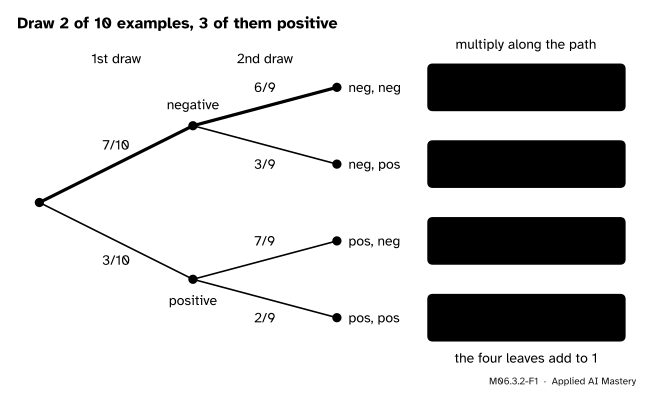
Two draws without replacement. The branches of the second draw change with the first: after a negative, 6 of the 9 examples left are negative. The chance of a whole path is the product of its branches.
Read the thick path. The first draw is negative with chance \(7/10\). Given that, 9 examples are left and 6 of them are negative, so the second is negative with chance \(6/9\). Of all the ways the two draws can go, a share \(7/10\) starts with a negative, and a share \(6/9\)of those continues with another. A share of a share is a product: \({7/10 \times 6/9 = 7/15}\).
Build it up
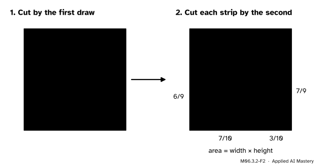
The same product is an area. Start with the unit square of all possibilities.
Step 1. Cut it into two strips by the first draw: a strip of width \(7/10\) for “first negative” and one of width \(3/10\) for “first positive”.
Step 2. Cut each strip across by the second draw, using the chances that hold inside that strip. In the left strip, \(6/9\) of the height is “second negative”; in the right strip, after a positive has gone, \(7/9\) is.
M06.3.2-F2
A tree is an area diagram in disguise. Each rectangle has the width of the first branch and the height of the second, so its area is their product.
Each rectangle’s area is the chance of its path, and the four rectangles tile the square, so their areas add to 1. That is the check that every tree passes: \({7/15} + {7/30} + {7/30} + {1/15} = {14/30} + {7/30} + {7/30} + {2/30} = {1}\).
The formal statement
The multiplication rule. Multiply both sides of the definition \({\Prob(A \mid B) = \Prob(A \cap B)/\Prob(B)}\) by \({\Prob(B)}\):
\[
\Prob(A \cap B) = \Prob(B)\,\Prob(A \mid B) .
\]
The definition with the roles of \(A\) and \(B\) swapped gives, in the same way, \({\Prob(A \cap B) = \Prob(A)\,\Prob(B \mid A)}\). Both are true, and you use whichever conditional probability you know. In a tree it is the one for the earlier stage first.
The chain rule. For three events, treat \({A_1 \cap A_2}\) as a single event and use the rule once:
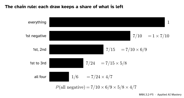
Every condition must have positive probability, so that each factor is defined. Each factor keeps a share of what was left after the factors before it.
M06.3.2-F5
The chain rule on the mini-batch. Each bar is the one above it times a conditional probability, so the shrinking happens one stage at a time.
Why a tree works. Each path of a tree is a chain of events, one per stage, so the chain rule says its chance is the product of its branches. At every fork the branches cover all the ways the stage can go, and none overlap, so they are a probability given the path so far and add to 1. The leaves therefore split all the probability without gaps or overlaps, and they add to 1.
Go deeper: the chain rule by induction
Write \(C_k\) for \({A_1 \cap \cdots \cap A_k}\). The claim for \(n\) events is
For \({n = 1}\) it reads \({\Prob(A_1) = \Prob(A_1)}\). Suppose it holds for \(n\). Since \({C_{n+1} = C_n \cap A_{n+1}}\), the multiplication rule gives \({\Prob(C_{n+1})} = {\Prob(C_n)\,\Prob(A_{n+1} \mid C_n)}\). Replace \({\Prob(C_n)}\) by its product of \(n\) factors and the claim for \({n + 1}\) appears. The assumption that \({\Prob(C_{n-1}) > 0}\) keeps every factor defined, and it also makes every earlier \(C_k\) positive, because \({C_{n-1}}\) lies inside each of them.
Worked example
The mini-batch, one draw at a time. Of 10 examples, 3 are positive and 7 negative. Four are drawn without replacement. Let \(N_k\) be the event “draw \(k\) is negative”. We want \({\Prob(N_1 \cap N_2 \cap N_3 \cap N_4)}\).
Stage by stage. Before the first draw, 7 of the 10 are negative. If the first was negative, 6 of the 9 left are. If the first two were, 5 of the 8 left are, and then 4 of the 7.
That is the \(1/6\) of M06.2.4, found without counting a single batch. The top line, \(840\) over \(5040\), is in fact a count: ordered draws of four negatives over all ordered draws of four.
M06.3.2-F3
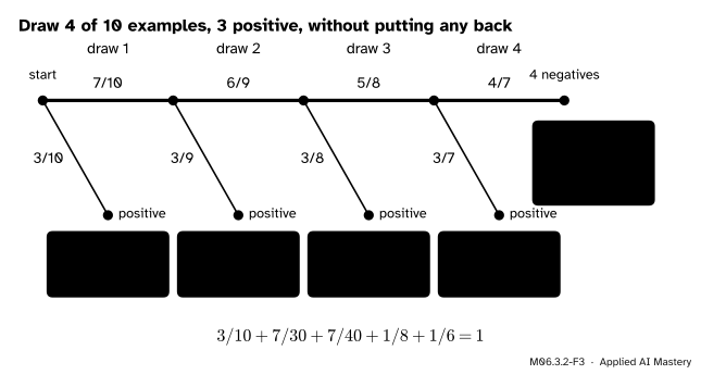
The tree of “when is the first positive drawn?”. Each side branch ends the moment a positive turns up. The five leaves are all the ways the batch can begin, so their chances add to 1.
Check with the leaves. The tree in the figure stops at the first positive. Its five leaves are “first positive at draw 1, 2, 3 or 4” and “no positive”. Over a common denominator of 120 their chances are \({36 + 28 + 21 + 15 + 20 = 120}\) parts, so they add to 1, as every tree’s leaves must.
Code
From scratch, with exact fractions: multiply the conditional chances stage by stage, then count ordered draws to confirm.
from fractions import Fractionfrom itertools import permutationsfrom math import proddef chance_no_positive(n_total, n_positive, k):"""Chain rule: at each draw, negatives left over examples left.""" negatives = n_total - n_positivereturn prod(Fraction(negatives - j, n_total - j) for j inrange(k))by_chain = chance_no_positive(10, 3, 4)labels = [1] *3+ [0] *7# 1 = positivedraws =list(permutations(range(10), 4)) # every ordered draw of 4none =sum(1for d in draws ifall(labels[i] ==0for i in d))print("chain rule:", by_chain, " counting:", none, "/", len(draws), "=", Fraction(none, len(draws)))
chain rule: 1/6 counting: 840 / 5040 = 1/6
The leaves of the “first positive” tree, built by the same rule:
leaves, alive = [], Fraction(1) # alive: chance that no positive has turned up yetfor j inrange(4): left, negatives =10- j, 7- j leaves.append(alive * Fraction(3, left)) # first positive at draw j + 1 alive *= Fraction(negatives, left)leaves.append(alive) # no positive at allprint([str(x) for x in leaves], " total:", sum(leaves))
['3/10', '7/30', '7/40', '1/8', '1/6'] total: 1
Now a simulation. rng.choice with replace=False draws a batch the way a data loader does.
The simulated share is close to \(1/6\); the last digits depend on the seed.
The same rule scores a sentence in a language model. The model gives the chance of each word given the words before it, and the chain rule multiplies them. The numbers below are invented for the example; a real model has a vocabulary of many thousands of words.
import math# invented conditional chances: P(first word), P(second | first), P(third | first two)steps = [("the", 0.06), ("cat", 0.01), ("sat", 0.05)]p_sentence = math.prod(p for _, p in steps)log_p =sum(math.log(p) for _, p in steps) # models add logs, so tiny products do not underflowprint(f"P(the cat sat) = {p_sentence:.2e} log = {log_p:.3f}")
P(the cat sat) = 3.00e-05 log = -10.414
Explore
This module’s interactive, the zoom-in square, lives in lesson M06.3.3. Its tree is the tree of this lesson with two stages, and its four areas are the four rectangles of the build-up figure. Move any slider and check that each leaf is the product of its two branches and that the leaves add to 1.
Pitfalls
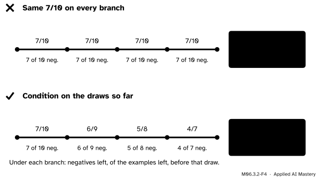
M06.3.2-F4
Wrong beside right. Using \(7/10\) at every draw pretends that each example is put back before the next draw. Without replacement the branches must follow the examples that are left.
“The chance of A and B is the chance of A times the chance of B.”
Only when learning one tells you nothing about the other, which is independence (M06.3.4). In general the second factor must be conditional. For the mini-batch, \({(7/10)^4 = 0.2401}\) is the answer for drawing with replacement; without replacement it is \({1/6 \approx 0.167}\).
“A branch carries the chance of reaching its end from the start.”
A branch carries a conditional probability: the chance of that step given the path before it. The chance of reaching a leaf from the start is the product along the path. Writing \(7/15\) on the second branch of the thick path would count the first draw twice.
“My tree’s leaves add to 0.9, but each branch looks right.”
Then a branch is missing, or a fork’s branches do not add to 1. At every fork the branches must cover every way the stage can go. Adding the leaves is the quickest check on a tree.
Check yourself
Recall
1. State the multiplication rule in both of its forms.
3. What number goes on a branch of a probability tree?
Show answer
The conditional probability of that step given the path that leads to its fork.
4. Why do the leaves of a probability tree add to 1?
Show answer
At each fork the branches add to 1, so splitting a path’s chance among its branches never loses or adds any. The leaves split the total of 1 without gaps or overlaps.
5. What is the chance that a mini-batch of 4 drawn without replacement from 10 examples, 3 positive, has no positive? Give the product.
1.★ Two cards are dealt from a well-shuffled deck of 52. Find the chance that both are hearts.
Show solution
\({\Prob(H_1) = 13/52}\) and, given a heart has gone, \({\Prob(H_2 \mid H_1) = 12/51}\). So \({\Prob(H_1 \cap H_2)} = {(13/52)(12/51)} = {156/2652} = {1/17}\).
2.★★ For the mini-batch, find the chance that the first two draws are positive and the next two are negative. Is it the same as the chance of negative, negative, positive, positive?
Show solution
Positive, positive, negative, negative: \({(3/10)(2/9)(7/8)(6/7)} = {252/5040} = {1/20}\). Negative, negative, positive, positive: \({(7/10)(6/9)(3/8)(2/7)} = {252/5040} = {1/20}\). The same: each product has \({3 \cdot 2}\) and \({7 \cdot 6}\) on top and \({10 \cdot 9 \cdot 8 \cdot 7}\) below, only in a different order. Every order of two positives and two negatives has chance \(1/20\), and there are \({\binom{4}{2} = 6}\) orders, so exactly two positives has chance \({6/20 = 3/10}\), which matches the count of M06.2.4, \({\binom{3}{2}\binom{7}{2}/\binom{10}{4} = 63/210}\).
3.★★★ An urn holds 2 red and 3 blue balls. A ball is drawn and put back together with one more ball of the same colour; then a second ball is drawn. Draw the tree, find the chance that the second ball is red, and compare it with the chance that the first is red.
Show solution
First draw: red \({2/5}\), blue \({3/5}\). After red the urn has 3 red and 3 blue, so red next has chance \({3/6}\); after blue it has 2 red and 4 blue, so red next has chance \({2/6}\). The two paths that end in a red second ball have chances \({(2/5)(3/6) = 6/30}\) and \({(3/5)(2/6) = 6/30}\). They are different leaves, so they add: \({12/30 = 2/5}\). The second ball is red with the same chance as the first, even though each branch changes. Adding leaves like this is the law of total probability, the next lesson.
Summary card
A share of a share is a product: multiply conditional probabilities along a path.
M06.3.2-F1
Branches are conditional; paths multiply.
Multiplication rule.\({\Prob(A \cap B) = \Prob(B)\,\Prob(A \mid B)}\).
Chain rule. Each factor is conditioned on all the events before it.
Trees. A branch holds a conditional probability; a leaf is the product of its path; the leaves add to 1.
Sources. Each was opened and checked against this lesson on 12 November 2026.
Jeremy Orloff and Jonathan Bloom, Reading 3: Conditional Probability, Independence and Bayes’ Theorem, MIT OpenCourseWare 18.05, Spring 2022. Section 3 states the multiplication rule as equation (2), a rewriting of the definition; section 5 builds trees with conditional probabilities on the branches and says the chance of reaching a node is the product along its path.
Charles M. Grinstead and J. Laurie Snell, Introduction to Probability, second edition. Section 4.1, Figure 4.1 and Example 4.5: a tree whose branch weights are conditional probabilities and whose paths carry their products.