Conditional probability: shrinking the sample space
Learning that an event B happened throws away every outcome outside B and shares the whole probability among the outcomes that are left. Define P(A | B), see why the order around the bar matters, and compute it on two dice and an inbox.
Define the conditional probability P(A | B) as P(A and B) divided by P(B), for P(B) > 0, and explain it as zooming in on B.
Compute a conditional probability by counting on an equally likely space and from a two-way table of counts.
Show that P( . | B) obeys the three axioms of probability, so every rule of probability holds inside B.
Tell P(A | B) from P(B | A) and from P(A and B), and say which total each one divides by.
Compute conditional probabilities in Python, first by filtering counts and then with pandas.crosstab and normalize.
In review. The maths and code on this page are checked by automated tests on every change, but an independent reader has not signed it off yet. Spot a mistake or a confusing step? Tell us.
The question
Out of 100 emails in an inbox, 40 are spam. A new email arrives and you have not opened it, so the chance that it is spam is 0.4. Then you see that it contains the word “free”. Now what is the chance that it is spam? A spam filter answers this question for every word of every email. What exactly does it compute, and why is it not the same as the chance that a spam email contains “free”?
Intuition
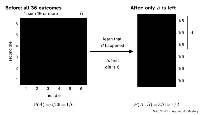
A probability always belongs to some set of possible outcomes. Before you learn anything, that set is the whole sample space \(\Omega\). When you learn that an event \(B\) has happened, every outcome outside \(B\) is ruled out. The outcomes inside \(B\) are all that is left, so they must now share the whole probability of 1 between them.
M06.3.1-F1
Roll two dice. Event \(A\) is “the sum is 10 or more” and event \(B\) is “the first die shows 6”. Before you know anything, \(A\) holds 6 of the 36 equally likely outcomes. Once you know \(B\) happened, only the six outcomes of \(B\) are left, each now worth \(1/6\), and three of them are in \(A\).
The picture shows the two moves of conditioning.
Throw away what cannot have happened. Only the outcomes in \(B\) survive.
Rescale what is left. The survivors keep their relative sizes but are blown up until they total 1.
The chance of \(A\) then is the share of \(B\) that lies in \(A\). On the dice it jumps from \(1/6\) to \(1/2\): knowing that the first die is a 6 makes a big sum much more likely.
Build it up
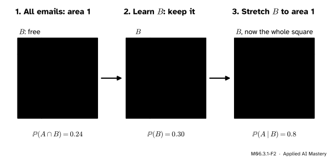
Counting cells works when every outcome is equally likely. Areas work always. Picture the sample space as a square of area 1, and each event as a region whose area is its probability (M06.1.3). Take the inbox: \(B\) is “contains free”, a strip of area 0.30, and \(A\) is “spam”.
Step 1. The overlap \(A \cap B\), spam that contains “free”, has area 0.24, since 24 of the 100 emails are both.
Step 2. Learn \(B\). Cross out everything outside the strip. What is left has area 0.30, not 1.
Step 3. Stretch the strip until it fills the square. Every part of it grows by the same factor, \({1/0.30}\), so the spam part grows from 0.24 to \({0.24/0.30 = 0.8}\).
M06.3.1-F2
Conditioning on \(B\) in three steps. The part of \(A\) inside \(B\) keeps its share of \(B\), and that share becomes the new probability of \(A\).
Stretching by \({1/\Prob(B)}\) is the whole idea. It turns a region of area \(\Prob(B)\) into a region of area 1, and it turns the overlap into a region of area \({\Prob(A \cap B)/\Prob(B)}\).
The formal statement
NoteDefinition: conditional probability
Let \(A\) and \(B\) be events with \({\Prob(B) > 0}\). The conditional probability of \(A\) given \(B\) is
\[
\Prob(A \mid B) = \frac{\Prob(A \cap B)}{\Prob(B)} .
\]
It is read “the probability of \(A\) given \(B\)”. The event after the bar is the condition.
If \({\Prob(B) = 0}\) the fraction has no meaning, and the definition says nothing.
On an equally likely space it is a count. When \(\Omega\) is finite and all its outcomes are equally likely, \({\Prob(E) = |E| / |\Omega|}\) for every event \(E\) (M06.2.1). Put that in the definition:
The \(|\Omega|\) cancels. Conditioning on \(B\) is counting as if \(B\) were the whole sample space, which is exactly what the anchor picture did: 3 of the 6 cells of \(B\).
\(\Prob(\,\cdot \mid B)\) is a probability. Fix \(B\) and let \(A\) vary. The rule that sends \(A\) to \({\Prob(A \mid B)}\) obeys the three axioms of M06.1.3, checked one at a time.
Never negative.\({\Prob(A \cap B) \ge 0}\) and \({\Prob(B) > 0}\), so the fraction is at least 0.
The whole space has probability 1. Since \({\Omega \cap B = B}\), \({\Prob(\Omega \mid B) = \Prob(B)/\Prob(B) = 1}\).
Additive. Let \(A_1\) and \(A_2\) be disjoint. Then \({A_1 \cap B}\) and \({A_2 \cap B}\) are disjoint too, and their union is \({(A_1 \cup A_2) \cap B}\). So
\[
\begin{aligned}
&\Prob(A_1 \cup A_2 \mid B) \\
&\quad= \frac{\Prob\big((A_1 \cap B) \cup (A_2 \cap B)\big)}{\Prob(B)} \\
&\quad= \frac{\Prob(A_1 \cap B) + \Prob(A_2 \cap B)}{\Prob(B)} \\
&\quad= \Prob(A_1 \mid B) + \Prob(A_2 \mid B).
\end{aligned}
\]
The second line is the additivity of \(\Prob\) itself. The same steps work for countably many disjoint events. Because the axioms hold, every rule that M06.1.4 derived from them holds inside \(B\) as well. For example, the complement rule becomes \({\Prob(A^c \mid B) = 1 - \Prob(A \mid B)}\).
The order around the bar matters. Both \({\Prob(A \mid B)}\) and \({\Prob(B \mid A)}\) have the same numerator, the overlap. They divide it by different totals:
\[
\begin{aligned}
\Prob(A \mid B) &= \frac{\Prob(A \cap B)}{\Prob(B)}, \\[4pt]
\Prob(B \mid A) &= \frac{\Prob(A \cap B)}{\Prob(A)} .
\end{aligned}
\]
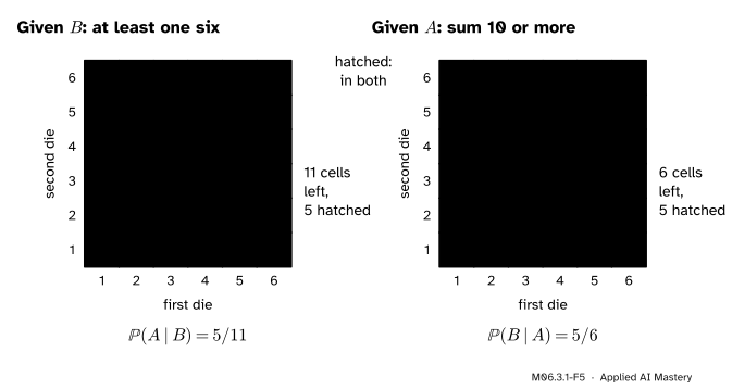
When the overlap has positive probability, they agree only when \({\Prob(A) = \Prob(B)}\). (When it has probability 0, both are 0.) Change the dice event \(B\) to “at least one die shows 6”.
M06.3.1-F5
The same five hatched outcomes are in both \(A\) and \(B\). Given \(B\) they are 5 of 11 cells; given \(A\) they are 5 of 6.
Go deeper: the conditional distribution, outcome by outcome
On a finite space we can condition one outcome at a time. Give each outcome \(\omega\) in \(B\) the new weight \({m(\omega \mid B) = m(\omega)/\Prob(B)}\) and each outcome outside \(B\) the weight 0. These new weights are never negative and add to \({\Prob(B)/\Prob(B) = 1}\), so they are a probability distribution on \(\Omega\), the conditional distribution given \(B\). Adding the new weights of the outcomes of \(A\) gives \({\Prob(A \cap B)/\Prob(B)}\), the definition again. Grinstead and Snell introduce conditional probability exactly this way. Every outcome in \(B\) keeps its size relative to the others: an outcome twice as likely as another before stays twice as likely after.
Worked example
The inbox. Of 100 emails, 40 are spam and 60 are not. The word “free” appears in 24 of the spam and in 6 of the others. One email is picked at random. Find the chance that it is spam given that it contains “free”, and the chance that it contains “free” given that it is spam.
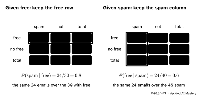
Lay the counts out as a table. The rows split the emails by the word, the columns by the label, and the totals sit at the edges: 30 contain “free”, 70 do not.
M06.3.1-F3
One table, read two ways. Conditioning on “free” keeps a row; conditioning on “spam” keeps a column. The overlap, 24 emails, is the numerator both times.
Given “free”. Learning that the email contains “free” keeps the 30 emails of the first row. Every email is equally likely to be the one picked, so
The same number from the definition, with probabilities in place of counts: \({\Prob(\text{spam} \cap \text{free}) = 0.24}\) and \({\Prob(\text{free}) = 0.30}\), so the ratio is \({0.24/0.30 = 0.8}\).
Given “spam”. Now the condition is the 40 spam emails of the first column:
The complement inside the condition. Since \({\Prob(\,\cdot \mid \text{free})}\) is a probability, \({\Prob(\text{not spam} \mid \text{free})} = {1} - {0.8} = {0.2}\), and the table agrees: 6 of the 30.
So seeing “free” moves the chance of spam from 0.4 to 0.8. A spam filter needs the first number, \({\Prob(\text{spam} \mid \text{free})}\). What it can count most easily in labelled data is the second, \({\Prob(\text{free} \mid \text{spam})}\), the share of known spam with the word. Getting from one to the other is Bayes’ rule, the subject of M06.4.
Code
First the dice, from scratch. Each event is a Python set of outcomes, and \({\Prob(A \mid B) = |A \cap B| / |B|}\) is one line.
from fractions import Fractionfrom itertools import productomega =set(product(range(1, 7), repeat=2)) # (first die, second die)A = {w for w in omega ifsum(w) >=10} # the sum is 10 or moreB = {w for w in omega if w[0] ==6} # the first die shows 6B2 = {w for w in omega if6in w} # at least one die shows 6def prob(event):return Fraction(len(event), len(omega))def cond(event, given):return Fraction(len(event & given), len(given))print("P(A) =", prob(A))print("P(A | B) =", cond(A, B))print("P(A | B2) =", cond(A, B2), " P(B2 | A) =", cond(B2, A))print("definition :", prob(A & B2) / prob(B2))
The count and the definition agree, as the cancelling of \(|\Omega|\) promised. Next the inbox, kept as a list of 100 records, one per email. Conditioning is filtering.
inbox = ([("spam", True)] *24+ [("spam", False)] *16+ [("not", True)] *6+ [("not", False)] *54)free = [label for label, has_free in inbox if has_free] # keep the conditionspam = [has_free for label, has_free in inbox if label =="spam"]p_spam_given_free = Fraction(free.count("spam"), len(free))p_free_given_spam = Fraction(sum(spam), len(spam))print(len(free), "emails with free;", "P(spam | free) =", p_spam_given_free)print(len(spam), "spam emails;", "P(free | spam) =", p_free_given_spam)
pandas does the same for a whole table at once. pandas.crosstab counts each pair of labels, and its normalize argument divides by a total: "index" divides each row by its row total, which is conditioning on the row, and "columns" divides each column by its column total.
import numpy as npimport pandas as pdemails = pd.DataFrame(inbox, columns=["label", "free"])counts = pd.crosstab(emails["free"], emails["label"])by_row = pd.crosstab(emails["free"], emails["label"], normalize="index") # given the wordby_col = pd.crosstab(emails["free"], emails["label"], normalize="columns") # given the labelprint(counts, "\n")print(by_row.round(3), "\n")print(by_col.round(3))# A simulation: pick 100,000 emails at random (with replacement) and keep those with 'free'.rng = np.random.default_rng(seed=3)picks = emails.iloc[rng.integers(0, 100, size=100_000)]share = (picks.loc[picks["free"], "label"] =="spam").mean()print("\nsimulated P(spam | free) =", round(share, 3))
Each row of by_row adds to 1, because each row is a probability distribution given that row’s condition. The simulated share lands close to 0.8; the exact digits depend on the seed.
Explore
This module’s interactive, the zoom-in square, lives in lesson M06.3.3. Choose the inbox preset there: the left strip is “spam” and its yellow part is “free”. The read-out turns the areas into \({\Prob(\text{spam} \mid \text{free})} = {0.24/0.30} = {0.8}\), the stretch of Step 3 above.
Pitfalls
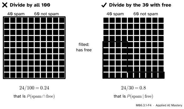
M06.3.1-F4
Wrong beside right. The numerator is the same 24 emails both times. Conditioning changes the denominator to the emails that are left.
“The chance it is spam and has ‘free’ is the chance it is spam given ‘free’.”
\({\Prob(A \cap B)}\) divides the overlap by everything; \({\Prob(A \mid B)}\) divides it by \(B\) alone. For the inbox the first is 0.24 and the second 0.8. A conditional probability is never smaller than the joint one, because it divides by \({\Prob(B) \le 1}\).
“P(spam | free) and P(free | spam) are two ways of writing the same thing.”
They share a numerator and divide it by different totals: 0.8 against 0.6 here, and 5/11 against 5/6 on the dice. With a rare condition the gap can be enormous. Confusing the two is the slip behind base-rate neglect (M06.4.2) and behind reading a classifier’s recall as its precision (ML01.7).
“Condition on anything, even an event that cannot happen.”
If \({\Prob(B) = 0}\) there is nothing left to rescale, and \({\Prob(A \mid B)}\) is undefined. In code this shows up as a division by zero, or as NaN in a table row with no entries. Check the size of the condition before dividing.
Check yourself
Recall
1. State the definition of \({\Prob(A \mid B)}\), with its condition on \(B\).
Show answer
\({\Prob(A \mid B) = \Prob(A \cap B)/\Prob(B)}\), defined when \({\Prob(B) > 0}\).
2. What two things happen to the outcomes when we condition on \(B\)?
Show answer
Every outcome outside \(B\) is thrown away, and the outcomes in \(B\) are rescaled by \({1/\Prob(B)}\) so that together they have probability 1.
3. On an equally likely space, what is \({\Prob(A \mid B)}\) as a count?
Show answer
\({|A \cap B| / |B|}\): the number of outcomes in both, over the number in \(B\).
4. In the inbox, what are \({\Prob(\text{spam} \mid \text{free})}\) and \({\Prob(\text{free} \mid \text{spam})}\)?
Show answer
\({24/30 = 0.8}\) and \({24/40 = 0.6}\).
5. Why does the complement rule hold for conditional probabilities?
Show answer
Because \({\Prob(\,\cdot \mid B)}\) obeys the three axioms, and the complement rule follows from the axioms alone. So \({\Prob(A^c \mid B) = 1 - \Prob(A \mid B)}\).
Exercises
1.★ Two dice are rolled. Find the probability that the sum is 8 given that both dice show an even number.
Show solution
Both even leaves \({3 \times 3 = 9}\) equally likely outcomes. Those with sum 8 are (2, 6), (4, 4) and (6, 2). So the answer is \({3/9 = 1/3}\), against \({5/36}\) before conditioning.
2.★★ In the inbox, find \({\Prob(\text{spam} \mid \text{no free})}\) and \({\Prob(\text{no free} \mid \text{not spam})}\). Then check that \({\Prob(\text{spam} \mid \text{free})}\) and \({\Prob(\text{spam} \mid \text{no free})}\) lie on either side of \({\Prob(\text{spam}) = 0.4}\).
Show solution
“No free” keeps the 70 emails of the second row, 16 of them spam: \({\Prob(\text{spam} \mid \text{no free})} = {16/70} = {8/35} \approx {0.229}\). “Not spam” keeps the 60 emails of the second column, 54 of them without the word: \({\Prob(\text{no free} \mid \text{not spam})} = {54/60} = {0.9}\). Seeing “free” raises the chance of spam to 0.8, and not seeing it lowers it to about 0.229; 0.4 lies between them. Lesson M06.3.3 shows that this always happens.
3.★★★ Show that if \(A\) lies inside \(B\) and \({\Prob(B) > 0}\), then \({\Prob(A \mid B)} = {\Prob(A)/\Prob(B)} \ge {\Prob(A)}\). When are the two equal? Check it with \(A\) = “double six” and \(B\) = “sum 10 or more”.
Show solution
If \(A\) lies inside \(B\) then \({A \cap B = A}\), so \({\Prob(A \mid B) = \Prob(A)/\Prob(B)}\). Since \({0 < \Prob(B) \le 1}\), dividing by \(\Prob(B)\) cannot make a non-negative number smaller, so \({\Prob(A \mid B) \ge \Prob(A)}\). They are equal when \({\Prob(A) = 0}\) or \({\Prob(B) = 1}\). For the dice, \({\Prob(\text{double six}) = 1/36}\) and \({\Prob(\text{sum} \ge 10) = 6/36}\), so the conditional probability is \({(1/36)/(6/36) = 1/6}\), six times larger.
Summary card
Conditioning on \(B\) throws away everything outside \(B\) and rescales what is left to total 1.
M06.3.1-F1
Keep \(B\), then share 1 among its outcomes.
Definition.\({\Prob(A \mid B) = \Prob(A \cap B)/\Prob(B)}\), for \({\Prob(B) > 0}\).
Still a probability.\({\Prob(\,\cdot \mid B)}\) obeys the axioms, so \({\Prob(A^c \mid B) = 1 - \Prob(A \mid B)}\).
Order matters. Same numerator, different totals: \({\Prob(\text{spam} \mid \text{free}) = 0.8}\), \({\Prob(\text{free} \mid \text{spam}) = 0.6}\).
Sources and next steps
Sources. Each was opened and checked against this lesson on 12 November 2026.
Charles M. Grinstead and J. Laurie Snell, Introduction to Probability, second edition (free under the GNU FDL). Section 4.1, Discrete Conditional Probability: the conditional distribution \({m(\omega_k \mid E) = m(\omega_k)/\Prob(E)}\) and the formula \({\Prob(F \mid E) = \Prob(F \cap E)/\Prob(E)}\), with the die of Example 4.1.
Jeremy Orloff and Jonathan Bloom, Reading 3: Conditional Probability, Independence and Bayes’ Theorem, MIT OpenCourseWare 18.05, Spring 2022. Equation (1) defines conditional probability; Example 10 shows how far apart \({\Prob(A \mid B)}\) and \({\Prob(B \mid A)}\) can be (1 against 1/16).
pandas developers, pandas.crosstab: the normalize argument, where "index" normalises over each row and "columns" over each column.