Independent variables have covariance 0, but zero covariance does not mean independence. Correlation sees only straight-line trends, one point can flip its sign, a shared cause creates it without causation, and from a few data points it strays a long way.
Prove that independent variables have covariance 0, and show with X uniform on −1, 0, 1 and Y = X² that the converse fails.
Recognise patterns that correlation cannot see: curves, circles and crossing lines, all with correlation 0.
Compute the sample covariance and the sample correlation r of n points by hand and with numpy.corrcoef and scipy.stats.pearsonr, and show how one outlier can flip the sign of r.
Explain, with a simulation, how a shared cause produces correlation without causation and how far r strays when n is small.
In review. The maths and code on this page are checked by automated tests on every change, but an independent reader has not signed it off yet. Spot a mistake or a confusing step? Tell us.
The question
A data scientist drops every input feature whose correlation with the target is close to 0, on the grounds that it is useless. A newspaper finds that towns which sell more ice cream have more sunburn, and asks whether ice cream should be taxed. Both lean on a correlation. What does a correlation of 0, or of 0.5, really tell you, and what can it not see at all?
From the last lesson
1. Between which values does \({\rho}\) lie, and when does it reach them?
Show answer
Between \({-1}\) and 1. It equals 1 or \({-1}\) exactly when \(Y\) is a straight-line function of \(X\), rising or falling.
2. What is the correlation of the course’s table?
Show answer
\({(1/4)/(1/2) = 1/2}\).
Intuition
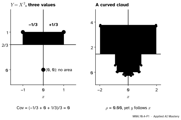
Let \(X\) be \({-1}\), 0 or 1 with chance \({1/3}\) each, and let \({Y = X^2}\). Once you know \(X\), you know \(Y\) exactly: the two are as dependent as variables can be. Now draw the rectangles of M06.10.1.
M06.10.4-F1
Left: the three values of \({(X, X^2)}\). The rectangles of the two outer points are mirror images, one green and one purple, and the middle point has none: the covariance is 0. Right: a noisy parabola. Every rectangle on one side has a mirror image of the opposite sign, so again the correlation is 0.
The mean of \(Y\) is \({2/3}\). The point \({(1, 1)}\) has deviations 1 and \({1/3}\): area \({+1/3}\). The point \({(-1, 1)}\) has deviations \({-1}\) and \({1/3}\): area \({-1/3}\). The point \({(0, 0)}\) sits on the mean of \(X\): area 0. They cancel exactly. Correlation asks one question, “does \(Y\) tend to rise or fall as \(X\) rises?”, and for a U shape the honest answer is neither.
Build it up
Step 1. Independence gives 0. If \(X\) and \(Y\) are independent, nothing about \(X\) shifts the balance of \(Y\), and the rectangles cancel. The proof is two lines, below.
Step 2. Zero does not give independence. The pair \({(X, X^2)}\) has covariance 0 and is completely dependent. Two variables with covariance 0 are called uncorrelated; uncorrelated is weaker than independent.
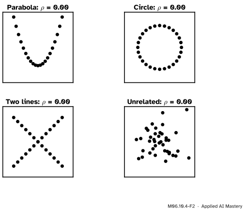
Step 3. Correlation sees only straight lines. A parabola, a circle, two crossing lines and a shapeless blob can all have correlation exactly 0.
M06.10.4-F2
Four clouds with correlation 0. Only the last has no relationship at all. In the other three \(y\) is tied to \(x\), but not by a straight line.
Step 4. One point can move it. A correlation is built from averages of products, and a point far from the others has a large product. The worked example shows a single point flipping the sign.
Step 5. A third variable can create it. If heat drives both ice-cream sales and sunburn, the two rise and fall together on hot and cool days though neither causes the other. The pitfalls section simulates exactly this.
The formal statement
NoteIndependence and correlation
If \(X\) and \(Y\) are independent, then \({\operatorname{Cov}(X, Y) = 0}\) and, when both standard deviations are positive, \({\rho(X, Y) = 0}\). The converse is false.
Proof. For independent variables \({\E[XY] = \E[X]\,\E[Y]}\) (M06.7.2). The shortcut of M06.10.1 then gives
and the correlation, the covariance divided by \({\sigma_X\sigma_Y}\), is 0 too.
The converse fails. Take \(X\) uniform on \({\{-1, 0, 1\}}\) and \({Y = X^2}\). Then \({\E[X] = 0}\). On these three values \({X^3 = X}\), so \({XY = X^3 = X}\) and \({\E[XY] = \E[X] = 0}\). Hence
Yet \({\Prob(X = 0, Y = 0) = \Prob(X = 0) = 1/3}\), while \({\Prob(X = 0)\,\Prob(Y = 0)}\)\({= \tfrac13 \cdot \tfrac13}\)\({= \tfrac19}\). One cell breaks the product rule, so they are not independent (M06.5.4).
From random variables to data. Given \(n\) points \({(x_i, y_i)}\), treat them as a distribution that puts probability \({1/n}\) on each point. Its means are the averages \(\bar x\) and \(\bar y\), and its covariance is the sample covariance
Its correlation is the sample correlation, written \(r\). Write \({dx_i = x_i - \bar x}\) and \({dy_i = y_i - \bar y}\). The factors \({1/n}\) cancel between the top and the bottom:
\[
r = \frac{\sum_i dx_i\, dy_i}{\sqrt{\sum_i dx_i^2\;\sum_i dy_i^2}} .
\]
Because \(r\) is the correlation of a distribution, everything in M06.10.3 holds for it: it lies between \({-1}\) and 1, ignores units, and is \({\pm 1}\) only when the points lie on a line. numpy.cov divides by \({n - 1}\) by default (S02.2 explains why); for \(r\) the divisor cancels, so it makes no difference.
Go deeper: what does zero correlation guarantee?
Exactly one thing: the best straight line for predicting \(Y\) from \(X\) is flat. By M06.10.3 its slope is \({\operatorname{Cov}/\operatorname{Var}(X) = 0}\), so the best line is the constant \({\mu_Y}\) and it removes none of the variance of \(Y\). A curve can still remove all of it, as \({y = x^2}\) does in the anchor figure. There is one family where zero correlation does force independence: jointly normal variables (M07.3), whose dependence is entirely straight-line. Indicators of two events are another (exercise 3 of M06.10.1).
Worked example
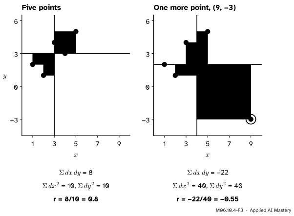
Five points by hand. Take \({(1, 2)}\), \({(2, 1)}\), \({(3, 4)}\), \({(4, 3)}\), \({(5, 5)}\). The means are \({\bar x = 15/5 = 3}\) and \({\bar y = 15/5 = 3}\).
point
\({dx}\)
\({dy}\)
\({dx\,dy}\)
(1, 2)
−2
−1
2
(2, 1)
−1
−2
2
(3, 4)
0
1
0
(4, 3)
1
0
0
(5, 5)
2
2
4
The products add to 8. The squares add to \({\sum dx^2}\)\({= 4 + 1 + 0 + 1 + 4}\)\({= 10}\) and \({\sum dy^2}\)\({= 1 + 4 + 1 + 0 + 4}\)\({= 10}\). So
One more point. Add \({(9, -3)}\), a typing slip perhaps. Now \({\bar x = 24/6 = 4}\) and \({\bar y = 12/6 = 2}\). The deviations are \({dx = -3, -2, -1, 0, 1, 5}\) and \({dy = 0, -1, 2, 1, 3, -5}\), so
\[
r = \frac{-22}{\sqrt{40 \times 40}} = -0.55 .
\]
M06.10.4-F3
The sample correlation by hand, before and after one extra point. The new point’s rectangle, of area \({5 \times (-5) = -25}\), outweighs all the others together and turns 0.8 into \({-0.55}\).
One point in six turned a clear rising trend into a falling one. Its deviations are large in both directions, and a product of two large numbers dominates the sum. Always plot the points before trusting an \(r\).
Code
The sample correlation from scratch, checked against numpy.corrcoef and scipy.stats.pearsonr (which also returns a p-value, a topic for S02.5).
five points: r = 0.8  numpy: 0.8  scipy: 0.8
six points:  r = -0.55
Y = X^2 on -1, 0, 1: covariance 0.0
Now two simulations. First the shared cause: heat \(Z\) drives both ice-cream sales and sunburn, each with its own independent noise, and neither affects the other. Then how far \(r\) strays from the true correlation 0 when the sample is small.
rng = np.random.default_rng(31)heat = rng.normal(size=600)ice_cream = heat + rng.normal(size=600)sunburn = heat + rng.normal(size=600)same_heat = np.abs(heat) <0.25print("all days: r =", round(sample_r(ice_cream, sunburn), 2)," days of nearly equal heat:", round(sample_r(ice_cream[same_heat], sunburn[same_heat]), 2))for n in (10, 100): a, b = rng.normal(size=(10_000, n)), rng.normal(size=(10_000, n)) a -= a.mean(axis=1, keepdims=True) b -= b.mean(axis=1, keepdims=True) r = (a * b).sum(axis=1) / np.sqrt((a * a).sum(axis=1) * (b * b).sum(axis=1))print(f"n = {n:3}: sd of r {r.std():.3f} (1/sqrt(n - 1) = {1/ np.sqrt(n -1):.3f}),"f" share with |r| >= 0.5: {np.mean(np.abs(r) >=0.5):.3f}")if n ==10: r10 = r
all days: r = 0.5   days of nearly equal heat: -0.08
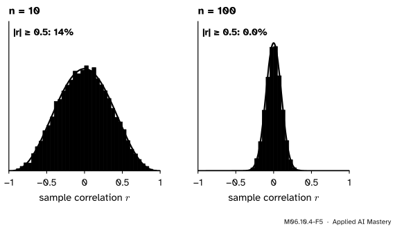
n =  10: sd of r 0.331 (1/sqrt(n - 1) = 0.333),  share with |r| >= 0.5: 0.138
n = 100: sd of r 0.101 (1/sqrt(n - 1) = 0.101),  share with |r| >= 0.5: 0.000
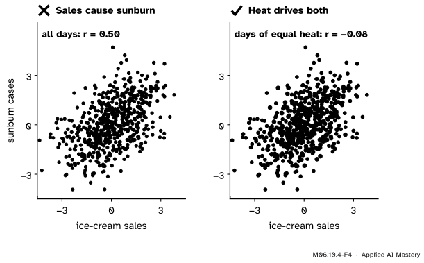
With 600 days the correlation is close to the \({1/2}\) that the set-up implies (exercise 3), yet among days of nearly equal heat it is close to 0. For pure noise, ten points give \({\abs{r} \ge 0.5}\) about one time in seven; a hundred points almost never do.
M06.10.4-F5
How far \(r\) strays when the true correlation is 0. With 10 points, about 14% of samples give \({\abs{r} \ge 0.5}\) (yellow); with 100 points the spread shrinks like \({1/\sqrt{n - 1}}\) and such values all but vanish.
Explore
Go back to the correlation explorer in M06.10.3 and try its two presets. Curved draws a cloud whose mass follows height along a U, with correlation exactly 0. One outlier adds a single mistyped person to a cloud of 29: set the slider to 0.6 and watch the outlier drag the correlation down to about 0.23.
Pitfalls
M06.10.4-F4
Wrong beside right. Over all days, sales and sunburn are clearly correlated. Hold the heat nearly fixed and the correlation all but vanishes: the shared cause made it.
“Correlation 0 means the feature is useless.”
It means the best straight line through the feature is flat. A target that depends on the size of a feature but not its sign, such as \({y = x^2}\), has correlation 0 with it and is still perfectly predictable. Screening features by correlation alone throws such features away; a scatter plot, or a model that can bend, keeps them.
“They are correlated, so one causes the other.”
A shared cause produces correlation with no causal link between the two. In the simulation heat drives both sales and sunburn and neither affects the other, yet \({r \approx 0.5}\) over all days. Holding the heat nearly fixed removes it. Confounding of this kind is the subject of S01.7, and causal inference (S06) studies when data can reveal cause at all.
“A correlation from ten points is as good as one from a thousand.”
A sample correlation is a random variable. From 10 points of pure noise it lands at 0.5 or beyond, in either direction, about 14% of the time. Before reading meaning into \(r\), ask how many points made it, and plot them: one outlier can flip its sign.
Check yourself
Recall
1. If \(X\) and \(Y\) are independent, what is their covariance, and why?
Show answer
0, because \({\E[XY] = \E[X]\,\E[Y]}\) for independent variables, and the shortcut subtracts exactly that.
2. Does covariance 0 imply independence? Give an example.
Show answer
No. With \(X\) uniform on \({\{-1, 0, 1\}}\) and \({Y = X^2}\) the covariance is 0, yet \(Y\) is fixed by \(X\).
3. What kind of relationship does correlation measure?
Show answer
Only straight-line association: how closely the points follow a rising or falling line.
5. How can two variables be correlated without either causing the other?
Show answer
A third variable, a shared cause, can drive both, as heat drives ice-cream sales and sunburn.
Exercises
1.★ Find the sample correlation of the points \({(1, 1)}\), \({(2, 3)}\), \({(3, 2)}\).
Show solution
\({\bar x = \bar y = 2}\). The deviations are \({dx = -1, 0, 1}\) and \({dy = -1, 1, 0}\), with products \({1, 0, 0}\), adding to 1. \({\sum dx^2 = 2}\) and \({\sum dy^2 = 2}\), so \({r = 1/\sqrt{2 \times 2}}\)\({= 1/2}\).
2.★★ Let \(X\) be uniform on \({\{-2, -1, 0, 1, 2\}}\) and \({Y = X^2}\). Show that \({\operatorname{Cov}(X, Y) = 0}\) and that \(X\) and \(Y\) are not independent.
Show solution
\({\E[X] = 0}\) by symmetry, and \({\E[XY] = \E[X^3]}\)\({= \tfrac15(-8 - 1 + 0 + 1 + 8)}\)\({= 0}\), so \({\operatorname{Cov}(X, Y) = 0 - 0 \cdot \E[Y] = 0}\). But \({\Prob(X = -2, Y = 0) = 0}\), while \({\Prob(X = -2)\,\Prob(Y = 0)}\)\({= \tfrac15 \cdot \tfrac15}\)\({= \tfrac{1}{25}}\). They differ, so the two are dependent.
3.★★★ Let \(Z\), \({E_1}\) and \({E_2}\) be independent, with \({\operatorname{Var}(Z) = s^2}\) and \({\operatorname{Var}(E_1) = \operatorname{Var}(E_2) = 1}\). Put \({X = Z + E_1}\) and \({Y = Z + E_2}\). Show that \({\rho(X, Y) = s^2/(s^2 + 1)}\), and evaluate it for the simulation, where \({s^2 = 1}\).
because independent variables have covariance 0. Independent variances add, so \({\operatorname{Var}(X)}\)\({= \operatorname{Var}(Y)}\)\({= s^2 + 1}\). Then \({\rho = s^2/\sqrt{(s^2 + 1)^2}}\)\({= s^2/(s^2 + 1)}\). With \({s^2 = 1}\) it is \({1/2}\): all of the correlation comes from the shared cause.
Summary card
Correlation sees straight lines, and nothing else.
M06.10.4-F1
Fully dependent, yet uncorrelated.
Independent \({\Rightarrow}\)\({\operatorname{Cov} = 0}\); the converse fails (\({Y = X^2}\)).
Curves, circles and crossing lines can all have \({\rho = 0}\).
\({r = \sum dx\,dy \big/ \sqrt{\sum dx^2 \sum dy^2}}\); one outlier can flip its sign (0.8 to \({-0.55}\)).
A shared cause gives correlation without causation.
For independent pairs, \(r\) has standard deviation \({1/\sqrt{n - 1}}\).
Sources and next steps
Sources. Each was opened and checked against this lesson on 12 November 2026.
Jeremy Orloff and Jonathan Bloom, Reading 7b: Covariance and Correlation, MIT OpenCourseWare 18.05, Spring 2022. Example 2 is exercise 2 of this lesson (\(X\) uniform on \({-2}\) to 2 and \({Y = X^2}\): covariance 0, not independent), with the remark that covariance measures only the linear relationship; Section 3.1 notes that correlation can completely miss higher-order relationships.
Hossein Pishro-Nik, Covariance and Correlation, Section 5.3.1 of Introduction to Probability, Statistics, and Random Processes: independent variables are uncorrelated, the converse fails, and a point chosen uniformly in the unit disc gives an uncorrelated but dependent pair.
SciPy, scipy.stats.pearsonr: the formula for \(r\), its range from \({-1}\) to 1, and, for independent normal samples, the beta distribution of \(r\) on \({[-1, 1]}\) with both shape parameters \({n/2 - 1}\), used here for the exact 14%.
NumPy, numpy.corrcoef: the correlation table, with entries between \({-1}\) and 1.
Next. M06.11, the law of large numbers and the central limit theorem, shows why averages of many independent draws settle down, which is also why the sample correlation steadies as \(n\) grows.