Correlation is the covariance of the two standardised variables, so no change of units can move it. One short calculation shows that it lies between −1 and 1, equals ±1 only for a straight line, and is the slope of the best line in standard units.
Define the correlation ρ = Cov(X, Y)/(σ_X σ_Y) as the covariance of the two standardised variables, and show that shifts and positive stretches leave it unchanged.
Derive E[(Z_Y − b Z_X)²] = 1 − 2bρ + b² and use it to prove that −1 ≤ ρ ≤ 1, with ±1 exactly for a straight line.
Find the slope of the best line, ρ in standard units and Cov/Var(X) in the original units, and the error it leaves, σ_Y²(1 − ρ²).
Compute ρ = 1/2 for the course’s table and check that its conditional means lie on the line of slope 1/2.
In review. The maths and code on this page are checked by automated tests on every change, but an independent reader has not signed it off yet. Spot a mistake or a confusing step? Tell us.
The question
Five people’s heights and masses have covariance 0.49 in metre kilograms, or 49 in centimetre kilograms. The two counts of the course’s table have covariance \({1/4}\), with no units at all. Which pair is more tightly tied? Covariance cannot say, because its size depends on the units. What number measures how closely two variables move together, the same in any units, and what does it have to do with fitting a straight line?
From the last lesson
1. State the variance of a sum for any \(X\) and \(Y\).
2. Two predictors’ errors each have variance \({\sigma^2}\) and covariance \(C\). What is the variance of the error of their average?
Show answer
\({(\sigma^2 + C)/2}\).
Intuition
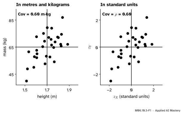
The units can be removed the way M06.7.4 removed them from one variable: standardise. Measure each height as a number of standard deviations from the mean height, and each mass as a number of standard deviations from the mean mass. The cloud does not move; only the numbers on the axes change.
M06.10.3-F1
The same 30 people before and after standardising. In standard units each axis counts standard deviations from its mean, the cloud has the same shape, and its covariance, now without units, is the correlation.
In standard units every variable has mean 0 and standard deviation 1, whatever it measured before. The covariance of the two standardised variables is therefore a pure number. That number is the correlation, written \({\rho}\) (the Greek letter rho).
Build it up
Step 1. Standardise. Write \({Z_X = (X - \mu_X)/\sigma_X}\) and \({Z_Y = (Y - \mu_Y)/\sigma_Y}\), each with mean 0 and variance 1 (M06.7.4).
Step 2. Take the covariance.\({Z_X}\) is \(X\) shifted by \({-\mu_X}\) and stretched by \({1/\sigma_X}\). By the rules of M06.10.2 the shift does nothing and the stretch scales, in each slot:
So the correlation is the covariance divided by the two standard deviations.
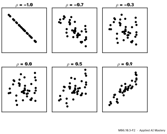
Step 3. See what the values look like. A correlation near 1 is a tight rising cloud, near \({-1}\) a tight falling one, and near 0 a shapeless blob.
M06.10.3-F2
Clouds of 40 points in standard units with six correlations. The sign gives the direction; the size says how closely the points hug a straight line, not how steep it is.
The formal statement
NoteDefinition: correlation
For \(X\) and \(Y\) with positive standard deviations,
Unchanged by units. Let \({a > 0}\) and \({c > 0}\). By the rules of M06.10.2, \({\operatorname{Cov}(aX + b, cY + d)}\)\({= ac\operatorname{Cov}(X, Y)}\), and by M06.7.3 the standard deviations become \({a\sigma_X}\) and \({c\sigma_Y}\). So
Metres or centimetres, kilograms or pounds: the correlation does not move. A negative \(a\) makes the standard deviation \({\abs{a}\sigma_X}\) while the covariance takes the sign of \(a\), so the correlation flips sign.
One calculation, three results. Try to predict \({Z_Y}\) by a multiple \({b\,Z_X}\) and look at the mean squared gap. Expand the square and use linearity:
The last line uses three facts. \({\E[Z^2] = \operatorname{Var}(Z) + (\E[Z])^2 = 1 + 0}\) for each standardised variable. And since both means are 0, the shortcut gives \({\E[Z_X Z_Y] = \operatorname{Cov}(Z_X, Z_Y) = \rho}\). Now complete the square in \(b\):
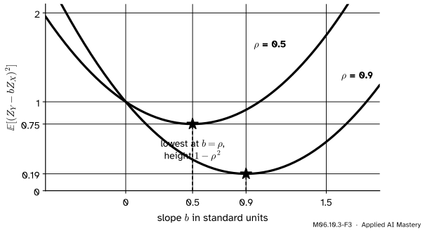
The mean squared gap \({1 - 2b\rho + b^2}\) as a function of \(b\), for \({\rho = 0.5}\) and \({\rho = 0.9}\). Each parabola is lowest at \({b = \rho}\), where it equals \({1 - \rho^2}\): 0.75 and 0.19.
Three results come out of that one line.
1. The correlation lies between \({-1}\) and 1. The left side is the expectation of a square, so it is never negative, whatever \(b\) is. Take \({b = \rho}\): then \({1 - \rho^2 \ge 0}\), which means \({\rho^2 \le 1}\), so \({-1 \le \rho \le 1}\).
2. It is \({\pm 1}\) exactly for a straight line. If \({\rho^2 = 1}\), the gap at \({b = \rho}\) is \({\E[(Z_Y - \rho Z_X)^2] = 0}\). A variable that is never negative and averages to 0 must be 0 on every outcome with positive probability. So \({Z_Y = \rho\,Z_X}\), which unpacks to
\[
Y = \mu_Y + \rho\,\frac{\sigma_Y}{\sigma_X}\,(X - \mu_X):
\]
a straight line, rising if \({\rho = 1}\) and falling if \({\rho = -1}\). Conversely, if \({Y = aX + b}\) with \({a \ne 0}\), the rule for units gives \({\rho(X, Y) = \pm\rho(X, X) = \pm 1}\), with the sign of \(a\).
3. It is the slope of the best line in standard units. Among all lines \({Z_Y \approx b\,Z_X}\), the mean squared gap is smallest at \({b = \rho}\), and the gap left over is \({1 - \rho^2}\). Turned back into the original units, the best line passes through the point of means with slope
This is the slope of least-squares regression (ML01.4.2), found here for a whole distribution. So \({\rho^2}\) is the share of the variance of \(Y\) that the best line accounts for, and \({1 - \rho^2}\) the share it leaves.
Go deeper: why the best line passes through the point of means
Allow an intercept: predict \({Z_Y}\) by \({b\,Z_X + k}\). The gap \({Z_Y - bZ_X}\) has mean 0, and for any variable \(G\) with mean 0, \({\E[(G - k)^2]}\)\({= \E[G^2] - 2k\,\E[G] + k^2}\)\({= \E[G^2] + k^2}\). That is smallest at \({k = 0}\). So in standard units the best line goes through the origin, which is the point of means, and only the slope is left to choose. (M06.7.4 found the same fact for a single guess: the best constant is the mean.)
Worked example
The course’s table. From M06.10.1 and M06.10.2: \({\operatorname{Cov}(X, Y) = 1/4}\) and \({\operatorname{Var}(X) = \operatorname{Var}(Y) = 1/2}\), so \({\sigma_X = \sigma_Y = \sqrt{1/2}}\) and
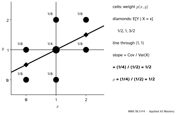
The best line. Its slope is \({\operatorname{Cov}/\operatorname{Var}(X)}\)\({= (1/4)/(1/2)}\)\({= 1/2}\), and it passes through the point of means \({(1, 1)}\): \({\hat y = 1 + \tfrac12(x - 1)}\)\({= \tfrac12 + \tfrac12 x}\).
The conditional means. In M06.9.3 each row of the table was rescaled into a PMF for \(Y\). Row \({x = 0}\) is \({(1/8, 1/8, 0)}\) out of \({1/4}\), so given \({X = 0}\), \(Y\) is 0 or 1 with chance \({1/2}\) each, and \({\E[Y \mid X = 0] = 1/2}\). The other rows give 1 and \({3/2}\). On the line, \({\hat y}\) is \({1/2}\), 1 and \({3/2}\) at \({x = 0, 1, 2}\): the conditional means lie exactly on it.
M06.10.3-F4
The course’s table as weighted points. The three conditional means (diamonds) lie on the line through the point of means with slope \({\operatorname{Cov}/\operatorname{Var}(X) = 1/2}\).
The error left over. The best line leaves mean squared error \({\sigma_Y^2(1 - \rho^2)}\)\({= \tfrac12 \cdot \tfrac34}\)\({= \tfrac38}\). Knowing \(X\) removes a quarter of the variance of \(Y\), which is \({\rho^2 = 1/4}\).
Code
First the course’s table with exact fractions. A square root of a fraction is not a fraction, so compute \({\rho^2}\) exactly and take the root at the end.
from fractions import Fractionfrom itertools import productimport mathjoint = {}for f1, f2, f3 in product([0, 1], repeat=3): joint[(f1 + f2, f2 + f3)] = joint.get((f1 + f2, f2 + f3), 0) + Fraction(1, 8)def E(g):returnsum(g(x, y) * p for (x, y), p in joint.items())mx, my = E(lambda x, y: x), E(lambda x, y: y)vx, vy = E(lambda x, y: (x - mx) **2), E(lambda x, y: (y - my) **2)c = E(lambda x, y: (x - mx) * (y - my))rho2 = c * c / (vx * vy)print("rho squared =", rho2, " rho =", math.sqrt(rho2), " slope Cov/Var(X) =", c / vx)line_mse = E(lambda x, y: (y - (my + c / vx * (x - mx))) **2)print("error left by the line:", line_mse, " = Var(Y)(1 - rho^2) =", vy * (1- rho2))
rho squared = 1/4   rho = 0.5   slope Cov/Var(X) = 1/2
error left by the line: 3/8   = Var(Y)(1 - rho^2) = 3/8
Now from data. numpy.corrcoef returns a table of correlations with 1 on the diagonal. Check that units do not matter, that a negative stretch flips the sign, and that the least-squares slope of numpy.polyfit is \({\operatorname{Cov}/\operatorname{Var}(X)}\).
Set the correlation with the slider and watch the rectangles: green ones grow as the cloud tilts up, purple ones as it tilts down. Then write the heights in centimetres, and compare the covariance and the correlation before and after.
Things to try. At a correlation of 1 every point is on a rising line and every rectangle is green. Switch to centimetres at any setting: the covariance is multiplied by exactly 100 and the correlation stays put. The two presets, a curved cloud and a single outlier, belong to the next lesson; try them now and see if you can predict what the read-out will say.
Pitfalls
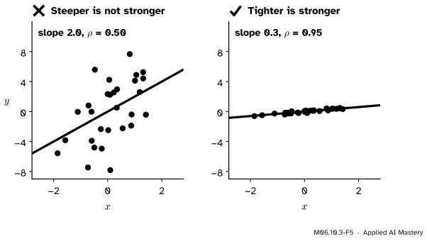
M06.10.3-F5
Wrong beside right. The steep cloud on the left has the weaker correlation. Correlation measures how tightly the points hug their line, not how steep the line is.
“A steeper line means a stronger correlation.”
The slope is \({\rho\,\sigma_Y/\sigma_X}\), so it mixes the correlation with the two spreads. A cloud can have slope 2 and correlation 0.5, and another slope 0.3 and correlation 0.95. Only in standard units is the slope the correlation.
“A correlation of 0.5 means the line explains half of the variation.”
The share of the variance of \(Y\) that the best line accounts for is \({\rho^2}\), so a correlation of 0.5 explains a quarter and leaves three quarters, as on the course’s table (\({3/8}\) out of \({1/2}\)). A correlation of 0.7 explains just under half.
“A correlation of 1 means the two variables are equal.”
It means that one is a straight-line function of the other with a positive slope. Temperature in Celsius and in Fahrenheit have correlation exactly 1, and they are never equal except at \({-40}\) degrees.
Check yourself
Recall
1. Define the correlation of \(X\) and \(Y\) in two ways.
Show answer
\({\rho = \operatorname{Cov}(X, Y)/(\sigma_X\sigma_Y)}\), which is also the covariance of the two standardised variables, \({\operatorname{Cov}(Z_X, Z_Y)}\).
2. What happens to \({\rho}\) when \(X\) is shifted, stretched by a positive number, or multiplied by \({-1}\)?
Show answer
A shift or a positive stretch leaves it unchanged; multiplying by \({-1}\) flips its sign.
3. Between which values does \({\rho}\) lie, and when does it reach them?
Show answer
Between \({-1}\) and 1. It equals 1 or \({-1}\) exactly when \(Y\) is a straight-line function of \(X\), rising or falling.
4. What is the slope of the best line for predicting \(Y\) from \(X\), in standard units and in the original units?
Show answer
\({\rho}\) in standard units, and \({\rho\,\sigma_Y/\sigma_X}\)\({= \operatorname{Cov}(X, Y)/\operatorname{Var}(X)}\) in the original units, through the point of means.
5. What is the correlation of the course’s table?
Show answer
\({(1/4)/(1/2) = 1/2}\).
Exercises
1.★\({\operatorname{Var}(X) = 4}\), \({\operatorname{Var}(Y) = 9}\) and \({\operatorname{Cov}(X, Y) = 3}\). Find \({\rho(X, Y)}\) and \({\rho(2X + 1, -Y)}\).
Show solution
\({\rho}\)\({= 3/(2 \times 3)}\)\({= 0.5}\). Stretching \(X\) by 2 and shifting it by 1 change nothing; multiplying \(Y\) by \({-1}\) flips the sign, so \({\rho(2X + 1, -Y) = -0.5}\).
2.★★ For the course’s table, find the correlation of \(X\) with \({X + Y}\).
Show solution
\({\operatorname{Cov}(X, X + Y)}\)\({= \operatorname{Var}(X) + \operatorname{Cov}(X, Y)}\)\({= 3/4}\) and \({\operatorname{Var}(X + Y) = 3/2}\) (M06.10.2). So
Square and take expectations. By the calculation in the lesson with \({b = \rho}\), \({\E[(Z_Y - \rho Z_X)^2] = 1 - \rho^2}\), so \({\E[(Y - \hat Y)^2] = \sigma_Y^2(1 - \rho^2)}\). For the course’s table this is \({\tfrac12 \cdot \tfrac34 = \tfrac38}\).
Summary card
Correlation is the covariance in standard units.
M06.10.3-F1
Same cloud, units divided out.
\({\rho = \operatorname{Cov}(X, Y)/(\sigma_X\sigma_Y)}\), which is \({\operatorname{Cov}(Z_X, Z_Y)}\).
Unchanged by shifts and positive stretches; \({-1 \le \rho \le 1}\).
Best slope: \({\operatorname{Cov}/\operatorname{Var}(X)}\), leaving \({\sigma_Y^2(1 - \rho^2)}\).
Course’s table:\({\rho = 1/2}\); conditional means on the line of slope \({1/2}\).
Sources and next steps
Sources. Each was opened and checked against this lesson on 12 November 2026.
Hossein Pishro-Nik, Covariance and Correlation, Section 5.3.1 of Introduction to Probability, Statistics, and Random Processes: the standardised variables of Equation 5.22, the correlation as their covariance, and a proof that \({-1 \le \rho \le 1}\) (by a different route, the inequality \({\alpha\beta \le (\alpha^2 + \beta^2)/2}\)), and that \({\rho = \pm 1}\) forces \({Y = aX + b}\).
Jeremy Orloff and Jonathan Bloom, Reading 7b: Covariance and Correlation, MIT OpenCourseWare 18.05, Spring 2022. Section 3.1 lists the properties (the covariance of the standardisations, dimensionless, between \({-1}\) and 1 with \({\pm 1}\) exactly for a line); Example 4 finds the correlation \({1/2}\) for the three-flip table; Section 4.2 proves the bound from \({\operatorname{Var}(X/\sigma_X - Y/\sigma_Y) \ge 0}\).
Chris Piech, Correlation, Probability for Computer Scientists: correlation as covariance normalised by the spread of each variable, measuring the degree of linear relationship.
NumPy, numpy.corrcoef: the correlation table is the covariance matrix divided by the square roots of its diagonal, with values between \({-1}\) and 1.
Next.M06.10.4 What correlation does not tell you shows dependent variables with correlation 0, an outlier that flips a correlation’s sign, and a shared cause that creates correlation without causation.