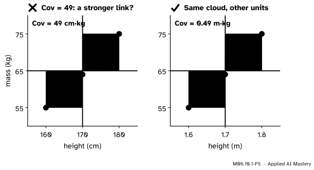
Covariance is the average product of two deviations from the means: positive in two quadrants, negative in the other two. Derive the shortcut E[XY] − E[X]E[Y], work it on the course’s joint table, and see why its size depends on the units.
Explain covariance as the average product of deviations, using the four quadrants cut by the two means.
Derive the shortcut Cov(X, Y) = E[XY] − E[X]E[Y] and compute E[XY] as a sum over the cells of a joint table.
Compute the covariance of the course’s joint table, 1/4, by the definition and by the shortcut, and show that Cov(X, X) = Var(X).
Compute a covariance from data, from scratch and with numpy.cov, and explain why its size alone says little.
In review. The maths and code on this page are checked by automated tests on every change, but an independent reader has not signed it off yet. Spot a mistake or a confusing step? Tell us.
The question
Taller people tend to be heavier. Houses with more rooms tend to cost more. A model’s error on one example tends to be large when its error on a similar example is large. In each case two random quantities move together, and in many others they pull in opposite directions. The variance of M06.7 measures how one variable spreads. What single number says whether two variables move together, and how strongly?
Intuition
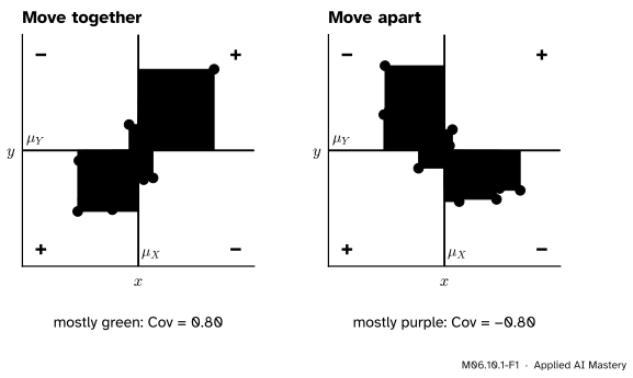
Draw a cloud of points, one per draw of the pair \({(X, Y)}\). Now draw two lines through the cloud: a vertical one at the mean of \(X\) and a horizontal one at the mean of \(Y\). They cut the plane into four quadrants.
For each point, measure how far it sits from each mean: its two deviations, \({x - \mu_X}\) and \({y - \mu_Y}\). Their product is the signed area of the rectangle that runs from the point of means to the point.
M06.10.1-F1
Each point’s rectangle runs from the crossing of the two means to the point. Up and right, or down and left, the product of deviations is positive (green, +). Up and left, or down and right, it is negative (purple, −). The covariance is the average signed area.
Two signs settle everything:
Up and to the right of both means, both deviations are positive, so the product is positive.
Down and to the left, both are negative, and the product is positive again.
In the other two quadrants one deviation is positive and one negative, so the product is negative.
When the variables move together, most points fall in the two positive quadrants and the green area wins. When they move apart, the purple area wins. When there is no pattern, the two roughly cancel. The average signed area is the covariance.
Build it up
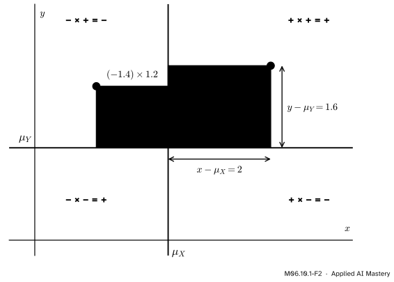
Step 1. One point, one rectangle. Take a point two units right of the mean of \(X\) and 1.6 units above the mean of \(Y\). Its rectangle has area \({2 \times 1.6 = 3.2}\), and it counts as positive. A point 1.4 units left and 1.2 units up has area \({(-1.4) \times 1.2 = -1.68}\).
M06.10.1-F2
One point’s rectangle. The signs of its two deviations fix the sign of its area: the rule of signs for multiplication, drawn as four quadrants.
Step 2. Weight and add. For a random pair, each possible point \({(x, y)}\) comes with a probability \({p(x, y)}\). Weight each rectangle’s signed area by its probability and add. That is an expectation: the expectation of the product of deviations.
Step 3. Read the sign. A positive total says that large values of \(X\) come with large values of \(Y\) more often than not. A negative total says the opposite. A total near 0 says that neither pattern dominates.
Step 4. Notice the units. If \(X\) is in metres and \(Y\) in kilograms, each area is in metre kilograms. Change metres to centimetres and every rectangle becomes 100 times wider. Hold that thought for the pitfalls.
The formal statement
NoteDefinition: covariance
For random variables \(X\) and \(Y\) on the same sample space, with means \(\mu_X\) and \(\mu_Y\),
So the covariance is the gap between the mean of the product and the product of the means. Here \({\E[XY]}\) is the expectation of a function of the pair, found as in M06.7.2 by weighting each cell:
\[
\E[XY] = \sum_x \sum_y xy\,p(x, y).
\]
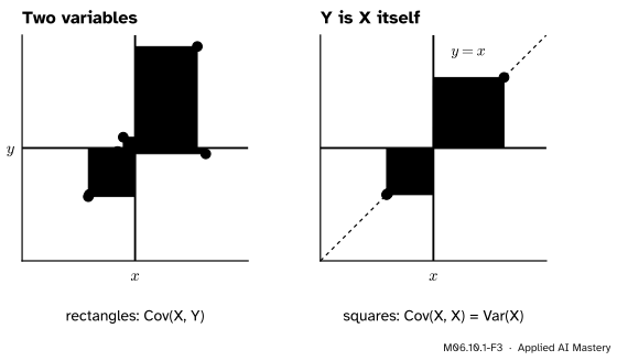
A variable with itself. Put \({Y = X}\). Every rectangle becomes a square, and
The variance is the covariance of a variable with itself, and the shortcut becomes the variance shortcut of M06.7.3, \({\E[X^2] - (\E[X])^2}\).
M06.10.1-F3
When \(Y\) is \(X\) itself, every point lies on the line \({y = x}\), every rectangle is a square, and every area is positive. The average area is the variance, the picture of M06.7.3 again.
Units. The covariance carries the product of the two units. Variance has squared units for the same reason. A covariance of 0.49 means nothing until you know whether it is in metre kilograms or centimetre kilograms. Lesson M06.10.3 divides the units out.
Go deeper: only one of the two variables needs centring
In the definition both variables are centred, but one is enough:
because \({\E[X - \mu_X] = \mu_X - \mu_X = 0}\). Centring the second variable as well changes no value of the sum; it only makes the picture symmetric. The shortcut is the case where neither is centred and the correction \({\mu_X \mu_Y}\) is paid at the end.
Worked example
The course’s joint table. Flip three fair coins. Let \(X\) be the number of heads among flips 1 and 2, and \(Y\) the number among flips 2 and 3. In eighths, the joint table (M06.9.1) is:
\({y = 0}\)
\({y = 1}\)
\({y = 2}\)
\({x = 0}\)
1
1
0
\({x = 1}\)
1
2
1
\({x = 2}\)
0
1
1
Both marginals are \({(1/4, 1/2, 1/4)}\), so \({\mu_X = \mu_Y = 1}\).
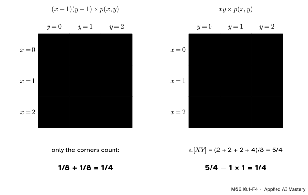
By the definition. The deviations are \({x - 1}\) and \({y - 1}\). Any cell in the middle row or the middle column has a deviation of 0, so its product is 0. That leaves the four corners. Two of them, \({(0, 2)}\) and \({(2, 0)}\), have probability 0. The other two each have product \({(-1)(-1) = (+1)(+1) = 1}\) and probability \({1/8}\):
so \({\operatorname{Cov}(X, Y)}\)\({= 5/4 - 1 \times 1}\)\({= 1/4}\). The two routes agree.
M06.10.1-F4
The covariance of the course’s table both ways. Left: the products of deviations, where only the two shaded corners count. Right: \({\E[XY] = 5/4}\), then subtract \({\mu_X \mu_Y = 1}\).
The covariance is positive because the counts share flip 2: a head there raises both. As a check of \({\operatorname{Cov}(X, X) = \operatorname{Var}(X)}\): \({\E[X^2]}\)\({= 0 \cdot \tfrac14 + 1 \cdot \tfrac12 + 4 \cdot \tfrac14}\)\({= \tfrac32}\), so \({\operatorname{Cov}(X, X)}\)\({= \tfrac32 - 1}\)\({= \tfrac12}\), the variance of a \({\text{Bin}(2, \tfrac12)}\) count.
Code
From scratch with exact fractions, by both routes.
from fractions import Fractionfrom itertools import product# The joint PMF, built from the 8 outcomes of three flips (1 = head).joint = {}for f1, f2, f3 in product([0, 1], repeat=3): key = (f1 + f2, f2 + f3) joint[key] = joint.get(key, 0) + Fraction(1, 8)def E(g):returnsum(g(x, y) * p for (x, y), p in joint.items())mx, my = E(lambda x, y: x), E(lambda x, y: y)cov_def = E(lambda x, y: (x - mx) * (y - my))exy = E(lambda x, y: x * y)print("means:", mx, my, " E[XY] =", exy)print("Cov by the definition:", cov_def, " by the shortcut:", exy - mx * my)print("Cov(X, X) =", E(lambda x, y: (x - mx) **2))
means: 1 1   E[XY] = 5/4
Cov by the definition: 1/4   by the shortcut: 1/4
Cov(X, X) = 1/2
Now from data. Simulate the three flips many times, and compute the average product of deviations, dividing by the number of draws \(n\). numpy.cov gives a whole table of covariances; with bias=True it divides by \(n\) like us, and by default it divides by \({n - 1}\), a choice S02.2 explains. For 100,000 draws the two hardly differ.
average product of deviations: 0.2491
numpy.cov, dividing by n:      0.2491
numpy.cov, dividing by n - 1:  0.2491
five people, metres:      0.49
five people, centimetres: 49.0
The simulated covariance lands within a hundredth of the exact \({1/4}\). The last two lines are the same five people, and the covariance is 100 times larger in centimetres.
Explore
This module’s interactive, the correlation explorer, lives in M06.10.3. It draws exactly the rectangles of this lesson for 30 points, totals the green and the purple, and lets you change the units of one axis, which is the subject of the pitfall below.
Pitfalls
M06.10.1-F5
Wrong beside right. The same five people with heights in centimetres (left) and in metres (right). The covariance is 100 times larger on the left, yet the cloud has not changed at all.
“A bigger covariance means a stronger relationship.”
The size of a covariance depends on the units. Five people of heights 1.60 to 1.80 m and masses 55 to 75 kg have covariance 0.49 metre kilograms. Write the same heights in centimetres and every deviation in height is 100 times larger, so the covariance is 49 centimetre kilograms. Nothing about the people changed. Only the sign of a covariance can be read on its own; to judge strength, divide out the units, which is what correlation does (M06.10.3). This matters whenever features in a data set have different units, which is why many methods standardise them first.
“The covariance is E[XY].”
Only when one of the means is 0. For the course’s table \({\E[XY] = 5/4}\), but the covariance is \({5/4 - 1 = 1/4}\). The mean of the product contains the product of the means, \({\mu_X \mu_Y}\), which says nothing about moving together. A pair of independent dice has \({\E[XY] = 12.25}\) (M06.7.2) and covariance 0.
“Covariance 0 means the variables have nothing to do with each other.”
It means the green and purple areas cancel. Independent variables do have covariance 0, but the reverse fails: the rectangles of a curved pattern can cancel exactly while one variable fixes the other. Lesson M06.10.4 builds such a pair.
Check yourself
Recall
1. Define the covariance of \(X\) and \(Y\).
Show answer
\({\operatorname{Cov}(X, Y)}\)\({= \E[(X - \mu_X)(Y - \mu_Y)]}\): the expected product of the two deviations from the means.
2. In which quadrants around the point of means is the product of deviations positive?
Show answer
Up and to the right (both deviations positive) and down and to the left (both negative). It is negative in the other two.
\({\operatorname{Var}(X)}\): with \({Y = X}\) every rectangle is a square.
5. Height is measured in centimetres and mass in kilograms. What are the units of their covariance, and what happens to it if heights are written in metres?
Show answer
Centimetre kilograms. In metres every height deviation is 100 times smaller, so the covariance is 100 times smaller too.
Exercises
1.★ Two variables take the values 0 and 1 with \({p(0, 0) = p(1, 1) = 0.4}\) and \({p(0, 1) = p(1, 0) = 0.1}\). Find their covariance.
Show solution
Both marginals give \({\Prob(X = 1) = \Prob(Y = 1) = 0.5}\), so \({\E[X] = \E[Y] = 0.5}\). The product \(XY\) is 1 only in the cell \({(1, 1)}\), so \({\E[XY] = 0.4}\). Then \({\operatorname{Cov}(X, Y)}\)\({= 0.4 - 0.5 \times 0.5}\)\({= 0.15}\). Positive: the two tend to agree.
2.★★ Roll one die. Let \(X\) be the top face and \({Y = 7 - X}\) the bottom face. Using \({\E[XY] = 28/3}\) from M06.7.2, find \({\operatorname{Cov}(X, Y)}\) and compare it with \({\operatorname{Var}(X) = 35/12}\).
It is exactly \({-\operatorname{Var}(X)}\). Every point lies on the falling line \({y = 7 - x}\), so every rectangle is purple. (Lesson M06.10.2 gives the quick reason: \({\operatorname{Cov}(X, 7 - X) = -\operatorname{Cov}(X, X)}\).)
3.★★★ For events \(A\) and \(B\), let \({I_A}\) and \({I_B}\) be their indicators. Show that \({\operatorname{Cov}(I_A, I_B)}\)\({= \Prob(A \cap B) - \Prob(A)\,\Prob(B)}\), and deduce that the covariance is 0 exactly when \(A\) and \(B\) are independent.
Show solution
An indicator’s expectation is the probability of its event (M06.7.1), so \({\E[I_A] = \Prob(A)}\) and \({\E[I_B] = \Prob(B)}\). The product \({I_A I_B}\) is 1 exactly when both events happen, so it is the indicator of \({A \cap B}\), and \({\E[I_A I_B] = \Prob(A \cap B)}\). The shortcut gives
This is 0 exactly when \({\Prob(A \cap B) = \Prob(A)\,\Prob(B)}\), which is the definition of independent events (M06.3.4). For indicators, unlike for variables in general, covariance 0 does mean independence.
Summary card
Covariance is the average signed rectangle of deviations.
Units: the product of the two units, so only the sign reads on its own.
Sources and next steps
Sources. Each was opened and checked against this lesson on 12 November 2026.
Hossein Pishro-Nik, Covariance and Correlation, Section 5.3.1 of Introduction to Probability, Statistics, and Random Processes: the definition and the shortcut \({E[XY] - (EX)(EY)}\), the reading of a positive and a negative covariance, and Lemma 5.3, whose first item is \({\operatorname{Cov}(X, X) = \operatorname{Var}(X)}\).
Jeremy Orloff and Jonathan Bloom, Reading 7b: Covariance and Correlation, MIT OpenCourseWare 18.05, Spring 2022. Section 2 defines covariance and lists its properties; Example 1 is this lesson’s table (three flips, the middle one shared) and finds the covariance \({1/4}\) by the definition, with only the two corners counting, and by \({\E[XY] = 5/4}\).
NumPy, numpy.cov: the default divides by \({N - 1}\), and bias=True divides by \(N\); two 1-D inputs give a 2 by 2 matrix.