Count what backpropagation costs: two matrix products backward for every one forward, so a gradient costs about three forward passes whatever the number of weights. Then the price in memory, checkpointing, and why the gradient shrinks or grows geometrically through twenty layers.
M05.9.4L2 Intermediate25 minIn review (what this means)
The maths and code on this page are checked by automated tests on every change, but an independent reader has not signed it off yet. Spot a mistake or a confusing step? Tell us.
Count the multiply-adds of the forward and backward pass of a dense network and explain why the backward pass costs at most about twice the forward pass.
Explain why backpropagation stores every activation, and derive the square-root memory of checkpointing.
Show that the adjoint reaching an early layer is a product of layer Jacobians whose norms multiply, and predict its geometric shrinking or growth from the weight scale.
Measure operation counts, checkpointed gradients and adjoint norms on a 20-layer NumPy network.
The question
Every training step of a deep network computes the gradient of the loss for every weight, perhaps a hundred million of them. Finite differences would need two hundred million runs of the network. What does backpropagation actually cost, in arithmetic and in memory? And when the gradient reaches the first of twenty layers, is it still the size it was at the top?
From the last lesson
1. What relative error do you expect from a correct backward pass checked in float64?
Show answer
About \({10^{-7}}\) or less; for the XOR network, near \({10^{-10}}\).
2. Why should a gradient check avoid ReLU kinks?
Show answer
The loss has no derivative there: the central difference straddles the kink and measures an average slope, so correct code can fail the check.
Intuition
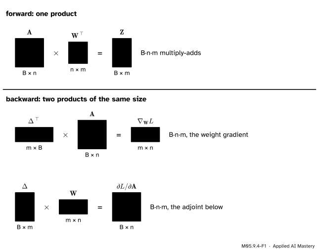
Almost all the arithmetic of a dense network is in its matrix products. A layer’s forward pass is one product. Its backward pass, from M05.9.2, needs two: one for the weight gradient and one for the adjoint it passes down. Both have the same three dimensions as the forward product.
M05.9.4-F1
One dense layer with a batch of \(B\) examples, \(n\) inputs and \(m\) outputs. The forward product and the two backward products each take \({B \cdot n \cdot m}\) multiply-adds, so backward costs twice forward.
So the gradient of all the weights costs about three forward passes: one forward, two backward. That is the constant of reverse mode in M05.8.4, made concrete. The number of weights does not appear. The price is memory: the product \({\mat{\Delta}\T\mat{A}}\) needs \(\mat{A}\), the layer’s input, so every layer’s input must still be there when the backward pass arrives.
Build it up
Step 1. Count one product. An \({m \times q}\) matrix times a \({q \times p}\) matrix computes \(mp\) entries, each a dot product of length \(q\): \({mpq}\) multiply-adds.
Step 2. Count a layer. Forward, \({\mat{A}\mat{W}\T}\) is \({(B \times n)(n \times m)}\): \({Bnm}\). Backward, \({\mat{\Delta}\T\mat{A}}\) is \({(m \times B)(B \times n)}\) and \({\mat{\Delta}\mat{W}}\) is \({(B \times m)(m \times n)}\): \({Bnm}\) each. The activation and its slope add only \({Bm}\) operations, a factor \(n\) fewer.
Step 3. Count a network. Add the layers, but note one saving: the first layer’s input is the data, whose adjoint nobody needs, so its backward pass is one product, not two.
M05.9.4-F2
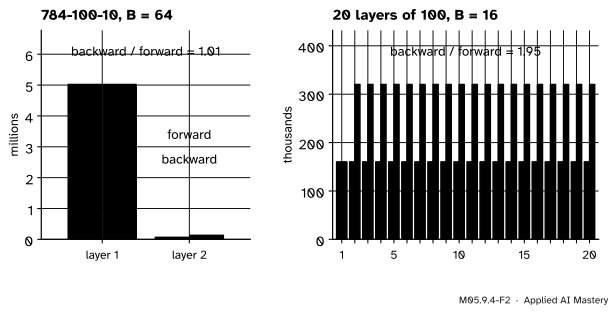
Multiply-adds layer by layer. In the deep network every layer but the first costs twice as much backward as forward. In the digit classifier almost all the work is in the first layer, whose input needs no adjoint, so backward costs barely more than forward.
Step 4. Memory. The backward pass of layer \(l\) needs \({\mat{A}^{(l-1)}}\) for the weight gradient and the slope \({1 - \mat{A}^{(l)} \odot \mat{A}^{(l)}}\) for the adjoint. Both were computed on the way forward, so the forward pass keeps every activation: \({L + 1}\) matrices of size batch times width for \(L\) layers. This is the tape of M05.8.3, one matrix per layer.
Step 5. The adjoint through depth. Each layer multiplies the adjoint by \({\mat{W}^{(l)}}\) and then entry by entry by a slope at most 1. Twenty layers make twenty such factors, and a product of twenty numbers each a little below 1, or a little above, is very small, or very large.
The formal statement
NoteCost, memory and the product of Jacobians
For a chain of \(L\) dense layers of widths \({n_0, n_1, \dots, n_L}\) and a batch of \(B\):
Cost. The forward products take \({F = B\sum_l n_{l-1} n_l}\) multiply-adds, and the backward products \({2F - B\,n_0 n_1}\), at most \(2F\).
Memory. Storing every activation takes \({L + 1}\) matrices. Keeping only every \(k\)-th as a checkpoint and recomputing each segment during the backward pass takes about \({L/k + k}\), least at \({k = \sqrt{L}}\), where it is \({2\sqrt{L}}\), for one extra forward pass.
Gradient flow. Per example, the adjoints obey \({\vect{\delta}^{(l-1)}} = {\mat{D}^{(l-1)}\mat{W}^{(l)\top}\vect{\delta}^{(l)}}\) with \({\mat{D}^{(l-1)}} = {\operatorname{diag}(1 - \vect{a}^{(l-1)} \odot \vect{a}^{(l-1)})}\), so
Cost. Layer \(l\) costs \({B n_{l-1} n_l}\) forward and twice that backward (Step 2), except layer 1, which skips \({\mat{\Delta}^{(1)}\mat{W}^{(1)}}\) (Step 3) and so saves \({B n_0 n_1}\). Adding over the layers gives the two totals.
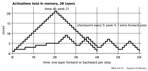
Memory. With checkpoints every \(k\) layers there are about \({L/k}\) of them. The backward pass handles one segment at a time: recompute its \(k\) activations from the checkpoint before it, run the backward pass through it, and free them. At most \({L/k + k}\) matrices are held at once. As a function of \(k\), \({f(k) = L/k + k}\) has \({f'(k) = 1 - L/k^2}\), which is zero at \({k = \sqrt{L}}\), and \({f(\sqrt{L})} = {\sqrt{L}} + {\sqrt{L}} = {2\sqrt{L}}\). Each layer’s forward step is recomputed once, which is one extra forward pass in all.
M05.9.4-F3
Memory over one training step of a 20-layer network. Keeping everything peaks at 21 stored activations. Checkpointing every fifth keeps 4 checkpoints and recomputes one segment at a time: the peak drops to 9, and the step takes 20 extra layer evaluations.
Gradient flow. The recurrence is M05.9.2’s batch rule for one row, with the entrywise product written as a diagonal matrix. Each step is a matrix times a vector, and the operator 2-norm satisfies \({\norm{\mat{M}\vect{v}}} \le {\norm{\mat{M}}_2\norm{\vect{v}}}\) and is submultiplicative, \({\norm{\mat{A}\mat{B}}_2} \le {\norm{\mat{A}}_2\norm{\mat{B}}_2}\) (M03.8.1). The diagonal entries \({1 - a^2}\) lie in \({(0, 1]}\), so \({\norm{\mat{D}^{(l-1)}}_2 \le 1}\), and \({\norm{\mat{W}^{(l)\top}}_2} = {\norm{\mat{W}^{(l)}}_2}\). Applying the bound \({L - 1}\) times gives the product. The adjoint at layer 1 is the top adjoint multiplied by \({L - 1}\) layer Jacobians, the product of Jacobians of M05.4.3, so its size is bounded by the product of their sizes.
Random weights. Draw the entries of a \({w \times w}\) matrix \(\mat{W}\) independently with mean 0 and variance \({s^2/w}\). For a fixed \(\vect{v}\), entry \(j\) of \({\mat{W}\T\vect{v}}\) is \({\sum_i W_{ij} v_i}\), a sum of independent terms with mean 0, so its expected square is the sum of their variances, \({\sum_i v_i^2 s^2/w} = {s^2\norm{\vect{v}}^2/w}\). Adding the \(w\) entries,
So each layer multiplies the adjoint’s size by about \(s\), times the typical slope \({1 - a^2}\). While the activations are small, the slopes are near 1 and the factor is about \(s\): below 1 the adjoint shrinks geometrically, above 1 it grows until tanh saturates and the slopes pull it back. This is the vanishing and exploding gradient problem, which DL02.4 treats in depth.
Go deeper: the weight gradients can stay balanced while the adjoints vanish
The weight gradient of layer \(l\) is \({\mat{\Delta}^{(l)\top}\mat{A}^{(l-1)}}\): an adjoint that shrinks going down times an activation that, for small weights, shrinks going up. In the linear regime, with layers of equal width and equal weight scale, the two rates cancel, and Glorot and Bengio (section 4.2.1) find the variance of the weight gradients the same in every layer while the variance of the back-propagated gradients may vanish or explode. Their remedy, the normalised initialisation, chooses the weight scale so that each layer approximately keeps both variances; DL02.3 develops it.
Worked example
Cost. For the digit classifier 784-100-10 with \({B = 64}\): forward \({64 \times (784 \times 100 + 100 \times 10)} = {5{,}081{,}600}\) multiply-adds. Backward: layer 2 needs \({2 \times 64{,}000}\), layer 1 only its weight gradient, \({5{,}017{,}600}\); in all \({5{,}145{,}600}\), about 1.01 times forward. For 20 layers of width 100 with \({B = 16}\), each layer costs \({16 \times 100 \times 100} = {160{,}000}\) forward, so \({3{,}200{,}000}\) in all, and backward \({2 \times 3{,}200{,}000 - 160{,}000} = {6{,}240{,}000}\): 1.95 times forward.
Memory. The 20-layer network keeps 21 activation matrices of \({16 \times 100}\). With a checkpoint every 5 layers it holds at most 9, and recomputes 20 layer evaluations.
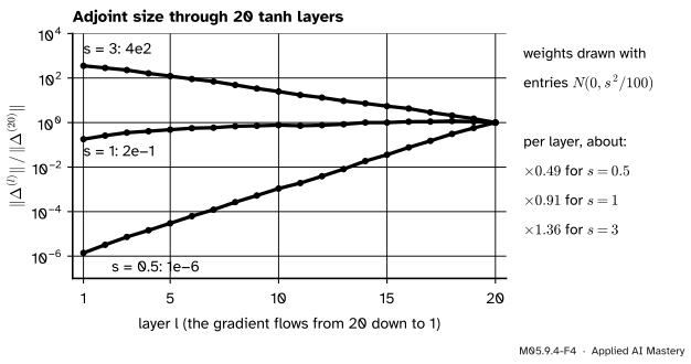
Gradient flow. Draw the weights of the 20-layer network with \({s = 0.5}\), \({s = 1}\) and \({s = 3}\), and follow the adjoint from the top layer down. The numbers depend on the random draw; these are for the seed in the code below.
M05.9.4-F4
The size of the adjoint, layer by layer, relative to the top. On a log scale a geometric change is a straight line: about \({\times 0.49}\) per layer for \({s = 0.5}\), a factor of about a million over 19 layers.
With \({s = 0.5}\) the factor per layer is about 0.49, close to \(s\) because the activations are small and their slopes near 1: after 19 factors, \({0.49^{19}} \approx {1.3 \times 10^{-6}}\). With \({s = 1}\), \({\E[\norm{\mat{W}\T\vect{v}}^2]}\) keeps the size, but the slopes \({1 - a^2 < 1}\) take about 9 per cent per layer. With \({s = 3}\) the product grows by about 1.36 per layer, much less than 3, because the activations saturate and their slopes are small.
Code
From scratch: a chain of dense tanh layers with no biases, its forward pass storing every activation, and its backward pass, with a counter of multiply-adds in every matrix product.
import numpy as npdef matmul(P, Q, tally): tally[0] += P.shape[0] * P.shape[1] * Q.shape[1] # m q p multiply-addsreturn P @ Qdef forward(Ws, X, tally): A = [X]for W in Ws: A.append(np.tanh(matmul(A[-1], W.T, tally)))return Adef backward(Ws, A, G, tally):"""G is the adjoint of the top activation. Returns the weight gradients and every adjoint norm.""" grads, norms = [None] *len(Ws), [None] *len(Ws) Delta = G * (1- A[-1] **2)for l inreversed(range(len(Ws))): norms[l] = np.linalg.norm(Delta) grads[l] = matmul(Delta.T, A[l], tally)if l >0: # the data needs no adjoint Delta = matmul(Delta, Ws[l], tally) * (1- A[l] **2)return grads, np.array(norms)def deep_chain(s, depth=20, width=100, batch=16, seed=0): rng = np.random.default_rng(seed) Ws = [rng.normal(0.0, s / np.sqrt(width), (width, width)) for _ inrange(depth)] X = rng.normal(0.0, 1.0, (batch, width)) c = rng.normal(0.0, 1.0, width) # loss: the mean over the batch of c^T a^(20)return Ws, X, np.tile(c, (batch, 1)) / batchWs, X, G = deep_chain(1.0)fwd, bwd = [0], [0]A = forward(Ws, X, fwd)grads, norms = backward(Ws, A, G, bwd)print(f"forward {fwd[0]:,} multiply-adds, backward {bwd[0]:,}, ratio {bwd[0] / fwd[0]:.2f}")print(f"activations stored: {len(A)} matrices of shape {A[0].shape}")
forward 3,200,000 multiply-adds, backward 6,240,000, ratio 1.95
activations stored: 21 matrices of shape (16, 100)
Checkpointing: keep only every fifth activation on the way forward; on the way back, recompute each segment from its checkpoint, run the backward pass through it, and free it. The gradient must come out exactly the same.
def backward_checkpointed(Ws, X, G, k, tally): checkpoints, a, held, peak = {0: X}, X, 1, 1for l, W inenumerate(Ws, start=1): # forward: keep A_0, A_k, A_2k, ... a = np.tanh(matmul(a, W.T, tally))if l % k ==0and l <len(Ws): checkpoints[l] = a grads, Delta = [None] *len(Ws), Nonefor start insorted(checkpoints, reverse=True): # segments from the top down seg = [checkpoints[start]]for W in Ws[start:start + k]: # recompute the segment seg.append(np.tanh(matmul(seg[-1], W.T, tally))) peak =max(peak, len(checkpoints) +len(seg) -1)if Delta isNone: Delta = G * (1- seg[-1] **2)for j inreversed(range(len(seg) -1)): # backward through the segment l = start + j grads[l] = matmul(Delta.T, seg[j], tally)if l >0: Delta = matmul(Delta, Ws[l], tally) * (1- seg[j] **2)return grads, peakck = [0]grads_ck, peak = backward_checkpointed(Ws, X, G, 5, ck)same =all(np.allclose(g1, g2, rtol=1e-12, atol=1e-15) for g1, g2 inzip(grads, grads_ck))print(f"same gradient: {same}; peak activations held: {peak} instead of {len(A)}")print(f"multiply-adds: {ck[0]:,} instead of {fwd[0] + bwd[0]:,} (one extra forward pass)")
same gradient: True; peak activations held: 9 instead of 21
multiply-adds: 12,640,000 instead of 9,440,000 (one extra forward pass)
Gradient flow: the size of the adjoint at layer 1 relative to the top, for three weight scales.
ratios = {}for s in (0.5, 1.0, 3.0): Ws_s, X_s, G_s = deep_chain(s) A_s = forward(Ws_s, X_s, [0]) _, n = backward(Ws_s, A_s, G_s, [0]) ratios[s] = n[0] / n[-1]print(f"s = {s}: layer 1 / layer 20 = {ratios[s]:.1e}, about {ratios[s] ** (1/19):.2f} per layer")
s = 0.5: layer 1 / layer 20 = 1.4e-06, about 0.49 per layer
s = 1.0: layer 1 / layer 20 = 1.8e-01, about 0.91 per layer
s = 3.0: layer 1 / layer 20 = 3.6e+02, about 1.36 per layer
In PyTorch the same trade is torch.utils.checkpoint; P08.6 looks at how engines manage memory.
Explore
The module’s interactive, the Backprop stepper in M05.9.2, shows the two costs on a small scale. Step through one example: the forward pass fills four columns of values, the backward pass fills the same nodes again with adjoints, and each weight’s gradient needs a value recorded on the way forward. Then train and watch the gradients shrink as the loss falls.
Pitfalls
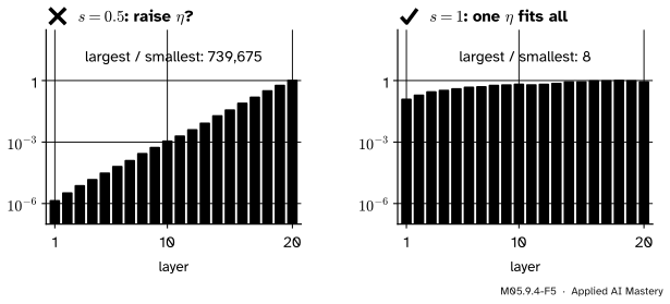
M05.9.4-F5
Wrong beside right. With \({s = 0.5}\) the gradients of the bias of layer 1 and layer 20 differ by a factor of about 740,000, so no single learning rate suits both. With \({s = 1}\) they differ by about 8.
“The first layer learns slowly, so raise the learning rate.”
Every layer shares one learning rate. A rate large enough for a gradient a million times smaller makes the top layers take steps a million times too large. The cure acts on the product itself: the weight scale (DL02.3), normalisation (DL02.5) or residual connections (DL02.7).
“Backpropagation costs about as much per weight as finite differences.”
Finite differences need two runs per weight. Backpropagation needs one forward and one backward pass for all of them, about three forward passes whatever the number of weights. For the 79,510 parameters of the digit classifier that is a factor of about 50,000.
“Free each activation as soon as the next layer has used it.”
The backward pass needs it again, for the weight gradient and the slope of the activation. Freeing it saves memory only if it is recomputed later, which is checkpointing: same gradient, one more forward pass.
“Checkpointing approximates the gradient.”
It recomputes exactly the same activations from exactly the same inputs, so the gradient is the same (the code asserts agreement to rounding). It trades time for memory, not accuracy.
Check yourself
Recall
1. How many matrix products does a dense layer need forward and backward?
Show answer
One forward; two backward (weight gradient and the adjoint passed down), each of the same size.
2. About how much does a full gradient cost, in forward passes?
Show answer
About three: one forward and about two backward, whatever the number of weights.
3. Why does backpropagation need memory for every layer’s activations?
Show answer
Each layer’s weight gradient \({\mat{\Delta}^{(l)\top}\mat{A}^{(l-1)}}\) needs its input, and the activation’s slope needs its output, both computed in the forward pass.
4. What does checkpointing every \(k\) of \(L\) layers cost and save?
Show answer
Memory about \({L/k + k}\) matrices instead of \({L + 1}\), least \({2\sqrt{L}}\) at \({k = \sqrt{L}}\), for one extra forward pass.
5. Why does the adjoint change geometrically with depth?
Show answer
It is multiplied by one layer Jacobian per layer, \({\mat{D}\mat{W}\T}\), and the sizes of these factors multiply; a factor of about \(s\) per layer gives about \({s^{L-1}}\).
Exercises
1.★ Count the multiply-adds of the matrix products of the XOR network 2-2-1 with the batch of 4, forward and backward. Why is the ratio not 2?
Show solution
Forward: \({4 \times 2 \times 2 = 16}\) for layer 1 and \({4 \times 2 \times 1 = 8}\) for layer 2, 24 in all. Backward: layer 2 needs its weight gradient and the adjoint below, \({2 \times 8 = 16}\); layer 1 needs only its weight gradient, 16, because the data needs no adjoint. In all 32, a ratio of \({4/3}\). The skipped product is a large share of a two-layer network; in a deep one it is one product among many.
2.★★ A network has \({L = 100}\) layers of equal width. Find the checkpoint spacing that minimises the number of stored activations, the number stored, and the total cost of a training step in forward-pass units, with and without checkpointing.
Show solution
\({f(k) = 100/k + k}\) is least at \({k = \sqrt{100} = 10}\): 10 checkpoints plus 10 activations of the segment in hand, 20 matrices instead of 101. Without checkpointing a step costs about 1 forward plus 2 backward, 3 units; with it, one more forward pass, about 4 units: a third more time for a fifth of the memory.
3.★★★ The entries of a \({w \times w}\) matrix \(\mat{W}\) are independent with mean 0 and variance \({s^2/w}\). Show that \({\E[\norm{\mat{W}\T\vect{v}}^2]} = {s^2\norm{\vect{v}}^2}\) for any fixed \(\vect{v}\). For a chain of linear layers (no activation), what is the expected squared size of the adjoint after 19 layers, and how does \({s = 0.5}\) compare with the measured tanh network?
Show solution
Entry \(j\) of \({\mat{W}\T\vect{v}}\) is \({\sum_i W_{ij} v_i}\). Its square has expectation \({\sum_i\sum_k v_i v_k\,\E[W_{ij}W_{kj}]}\), and by independence with mean 0 only the terms \({i = k}\) survive, each \({v_i^2\,s^2/w}\). So \({\E[(\mat{W}\T\vect{v})_j^2]} = {s^2\norm{\vect{v}}^2/w}\), and summing over the \(w\) entries gives \({s^2\norm{\vect{v}}^2}\). For independent layers, conditioning on the adjoint after each layer and applying this \({19}\) times gives \({\E[\norm{\vect{\delta}^{(1)}}^2]} = {s^{38}\norm{\vect{\delta}^{(20)}}^2}\), a typical size ratio of \({s^{19}}\). For \({s = 0.5}\) that is about \({1.9 \times 10^{-6}}\); the tanh network measured about \({1.4 \times 10^{-6}}\), a little smaller because its slopes \({1 - a^2}\) are slightly below 1.
Summary card
A gradient costs about three forward passes and a stored activation per layer.
M05.9.4-F1
One product forward, two back.
Backward multiply-adds \({2F - Bn_0n_1 \le 2F}\).
Memory: \({L + 1}\) activations; checkpointing \({2\sqrt{L}}\) for one extra forward pass.
Random weights of scale \(s\): about a factor \(s\) per layer while tanh is unsaturated.
Sources and next steps
Sources. Each was opened and checked against this lesson on 15 November 2026.
A. G. Baydin, B. A. Pearlmutter, A. A. Radul and J. M. Siskind, Automatic Differentiation in Machine Learning: a Survey, JMLR 18(153), 2018, section 3.2: reverse mode computes a gradient for \({c \cdot \text{ops}(f)}\) with \({c < 6}\) and typically 2 to 3, at the cost of storage that grows, in the worst case, with the number of operations, which checkpointing strategies reduce.
T. Chen, B. Xu, C. Zhang and C. Guestrin, Training Deep Nets with Sublinear Memory Cost, 2016. The abstract states \({O(\sqrt{n})}\) memory for an \(n\)-layer network for the cost of one extra forward pass per mini-batch; section 4.3, equation (1), divides the network into \(k\) segments for a memory cost of \({O(n/k) + O(k)}\), giving \({O(2\sqrt{n})}\) at \({k = \sqrt{n}}\).
X. Glorot and Y. Bengio, Understanding the difficulty of training deep feedforward neural networks, AISTATS 2010, section 4.2.1: in the linear regime, for layers of the same width and initialisation, the variance of the weight gradients is the same for all layers, while the variance of the back-propagated gradients may vanish or explode with depth; equation (16) is their normalised initialisation.
P. Bright, A. Edelman and S. G. Johnson, Matrix Calculus (for Machine Learning and Beyond), section 2.5.1: an \({m \times q}\) by \({q \times p}\) product takes \({mp}\) dot products of length \(q\), about \({2mpq}\) scalar operations.
Next. DL01.5 runs backpropagation by hand on larger networks, DL02.4 treats vanishing and exploding gradients in full, and P08.6 looks inside the engines that automate all of this.