When the inputs of a function themselves depend on other variables, the rate of change adds one product per path. Derive the multivariable chain rule from the linear approximation, draw it as a tree, and use it on the running bowl and the running loss.
M05.4.2L2 Intermediate25 minIn review (what this means)
The maths and code on this page are checked by automated tests on every change, but an independent reader has not signed it off yet. Spot a mistake or a confusing step? Tell us.
Derive dz/dt = f_x dx/dt + f_y dy/dt from the linear approximation, with the remainder handled.
Draw a tree diagram for variables that depend on one or several parameters, and read off each derivative as a sum over paths.
Apply the chain rule to the running bowl along a circle, to the bowl in polar coordinates and to a loss whose weight is a product of two numbers.
Explain why the derivative along a curve inside a level set is zero, and conclude that the gradient is perpendicular to the level set.
The question
A loss depends on the weights, but a weight is often computed from other numbers: two factors multiplied together, one number shared by two layers, a point that moves along a path as training runs. When those deeper numbers change, how fast does the loss change?
From the last lesson
1. A map has three inputs and two outputs. What shape is its Jacobian, and what is entry \({(2, 3)}\)?
Show answer
\(2 \times 3\). Entry \({(2, 3)}\) is \({\pd{f_2}{x_3}}\), the partial derivative of the second output in the third input.
2. What does the Jacobian of a map say about a small step \(\vect{h}\) from \(\vect{a}\)?
Show answer
The output moves by about \({\mat{J}_f(\vect{a})\,\vect{h}}\), with an error that is small even compared with \({\norm{\vect{h}}}\).
Intuition
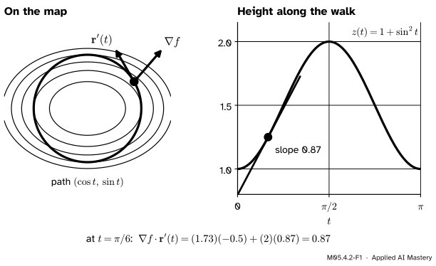
Walk anticlockwise round the unit circle on the map of the running bowl \({f(x, y) = x^2 + 2y^2}\). Your height \({z(t) = f(\cos t, \sin t)}\) changes because both coordinates change. Each one contributes its own slope times its own speed, and the two contributions add.
M05.4.2-F1
On the map, the rate of climb is the gradient dotted with the velocity. Along the walk, it is the slope of the height curve. Both give 0.87 at \({t = \pi/6}\).
So the rate of change is the gradient of \(f\) dotted with the velocity of the walker, \({\nabla f \cdot \vect{r}'(t)}\). The gradient says how steep each direction is; the velocity says which way and how fast you go.
Build it up
Step 1. A small change in the inputs. The linear approximation (M05.2.2) says that when \(x\) and \(y\) change by \({\Delta x}\) and \({\Delta y}\),
\[
\Delta z \approx \pd{f}{x}\,\Delta x + \pd{f}{y}\,\Delta y .
\]
Step 2. The inputs change because \(t\) does. If \({x = x(t)}\) and \({y = y(t)}\), a small change \({\Delta t}\) moves them by \({\Delta x \approx x'(t)\,\Delta t}\) and \({\Delta y \approx y'(t)\,\Delta t}\).
Step 3. Substitute and divide. Put Step 2 into Step 1 and divide by \({\Delta t}\):
As \({\Delta t \to 0}\) the left side becomes \({dz/dt}\). The formal statement makes the “about” exact.
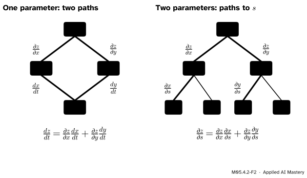
Step 4. Draw the dependencies as a tree. Put \(z\) at the top, the variables it depends on below, and their own variables below those. Write each branch’s derivative on it. The rule: multiply along each path from \(z\) down to the variable you want, and add the paths. With two parameters, follow only the branches that end at the one you are differentiating by.
M05.4.2-F2
Tree diagrams. Each path from the top to the variable you want contributes one product of branch derivatives; the paths add.
The formal statement
NoteThe chain rule
Let \({\vect{x}(t)}\) be a path in \(\R^n\) that is differentiable at \(t\), and let \(f\) be differentiable at \({\vect{x}(t)}\). Then \({z(t) = f(\vect{x}(t))}\) is differentiable at \(t\), and
where \({\rho(\vect{k})/\norm{\vect{k}} \to 0}\) and \({\rho(\vect{0}) = 0}\). Divide by \({\Delta t}\). The first term becomes \({\nabla f(\vect{a})\T (\vect{k}/\Delta t)}\), and \({\vect{k}/\Delta t \to \vect{x}'(t)}\) by the definition of the derivative of the path. For the second term, when \({\vect{k} \neq \vect{0}}\),
As \({\Delta t \to 0}\) the path is continuous, so \({\vect{k} \to \vect{0}}\) and the first factor tends to 0, while the second stays bounded, near \({\pm\norm{\vect{x}'(t)}}\). When \({\vect{k} = \vect{0}}\) the term is 0 anyway. So the second term tends to 0 and the formula follows. For several parameters, hold all but \(t_j\) fixed: then \({\vect{x}}\) is a path in \(t_j\) alone, and the same argument gives the second formula. ∎
Notice what the theorem needs: \(f\) differentiable, not merely with partial derivatives. The remainder argument is exactly where differentiability is used.
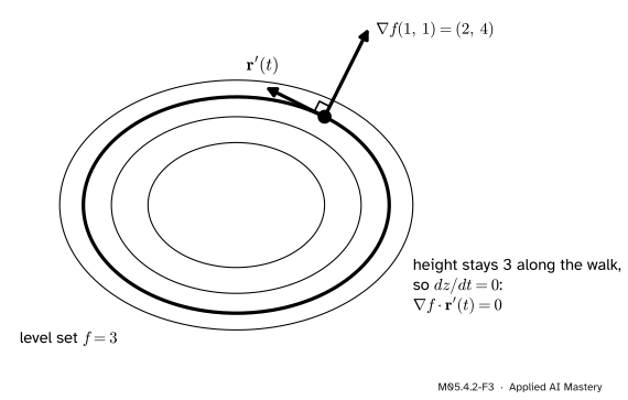
Gradients meet level sets at right angles. Let \({\vect{x}(t)}\) be a path that stays inside a level set \({f = c}\). Then \({z(t) = c}\) for every \(t\), so \({dz/dt = 0}\), and the chain rule says
\[
\nabla f(\vect{x}(t))\T\,\vect{x}'(t) = 0 .
\]
The velocity of any path in the level set is a tangent direction of that set, so the gradient is perpendicular to every tangent direction: a second proof of the result of M05.3.2.
M05.4.2-F3
A walk along the level set \({f = 3}\) keeps its height, so the chain rule gives \({\nabla f \cdot \vect{r}'(t) = 0}\): the gradient is perpendicular to the walk.
Worked example
The bowl round the circle. With \({x = \cos t}\) and \({y = \sin t}\), the partial derivatives \({f_x = 2x}\) and \({f_y = 4y}\) evaluated on the path are \({2\cos t}\) and \({4\sin t}\), and the velocity is \({(-\sin t, \cos t)}\). So
At \({t = \pi/6}\) this is \({2 \cdot \tfrac12 \cdot \tfrac{\sqrt3}{2} = \tfrac{\sqrt3}{2} \approx 0.866}\). Check by substituting first: \({z(t) = \cos^2 t + 2\sin^2 t = 1 + \sin^2 t}\), whose derivative is \({2\sin t\cos t}\), the same.
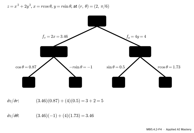
The bowl in polar coordinates. Now let \({x = r\cos\theta}\) and \({y = r\sin\theta}\), two parameters, and work at \({(r, \theta) = (2, \pi/6)}\), where \({x = \sqrt{3}}\) and \({y = 1}\). The top branches are \({f_x = 2\sqrt3 \approx 3.46}\) and \({f_y = 4}\). The lower branches are the entries of the polar Jacobian of lesson M05.4.1.
M05.4.2-F4
The worked example as a trace: every branch is a number, every path a product, and each derivative the sum of its two paths.
A loss with a factorised weight. Low-rank adapters and many other models write a weight as a product, \({w = uv}\). Take the running loss \({L(w, b)}\) of M04.10 with \({b = 0.5}\) held fixed, and \({u = 2}\), \({v = 0.5}\), so \({w = 1}\). The tree has one path from \(L\) through \(w\) to each factor:
The same product \({w = 1}\) gets pushes of different sizes on its two factors: each factor’s gradient is scaled by the other factor. Substituting first gives \({L = 7.5u^2v^2 - 21uv + 14.75}\), with \({\pd{L}{u} = 15uv^2 - 21v = -3}\) at this point, as claimed.
Frontier note: shared weights add paths
When one number is used in several places, the tree has several paths from the loss to it, and its derivative is the sum of their products. A recurrent network applies the same weight matrix at every time step, and a language model often uses one matrix both to embed words and to score them; in both cases the gradient of the shared weight is the sum of one contribution per use. Reverse-mode differentiation implements this rule by adding, not overwriting, the derivatives that arrive at a shared variable (M05.8.3), and forgetting to add them is a classic bug (M05.9.3).
Code
Each chain-rule answer is checked by differencing the composite function directly, without the chain rule.
import numpy as npdef bowl(x, y):return x **2+2* y **2def loss(w, b):return7.5* w **2+5* w * b + b **2-23.5* w -8* b +18.5def d(g, t, h=1e-6):"""Central difference of a function of one variable."""return (g(t + h) - g(t - h)) / (2* h)# 1. Along the circle, at t = pi/6.t0 = np.pi /6chain = (2* np.cos(t0)) * (-np.sin(t0)) + (4* np.sin(t0)) * np.cos(t0)direct = d(lambda t: bowl(np.cos(t), np.sin(t)), t0)print("circle:", round(chain, 6), round(direct, 6))# 2. In polar coordinates, at (r, theta) = (2, pi/6).r0, th0 =2.0, np.pi /6x0, y0 = r0 * np.cos(th0), r0 * np.sin(th0)dz_dr =2* x0 * np.cos(th0) +4* y0 * np.sin(th0)dz_dth =2* x0 * (-r0 * np.sin(th0)) +4* y0 * (r0 * np.cos(th0))z =lambda r, th: bowl(r * np.cos(th), r * np.sin(th))print("polar:", round(dz_dr, 6), round(d(lambda r: z(r, th0), r0), 6),round(dz_dth, 6), round(d(lambda th: z(r0, th), th0), 6))# 3. The loss with w = u v and b = 0.5, at (u, v) = (2, 0.5).u0, v0, b0 =2.0, 0.5, 0.5dL_dw =15* u0 * v0 +5* b0 -23.5print("factorised:", dL_dw * v0, round(d(lambda u: loss(u * v0, b0), u0), 6), dL_dw * u0, round(d(lambda v: loss(u0 * v, b0), v0), 6))
The direct differences agree with the chain rule to six decimal places in every case.
Explore
This module’s interactive, the grid warp, lives in lesson M05.4.1. Choose the polar map there and read the Jacobian at \({(2, 30^\circ)}\): its four entries are the four lower branches of the tree in the worked example.
Pitfalls
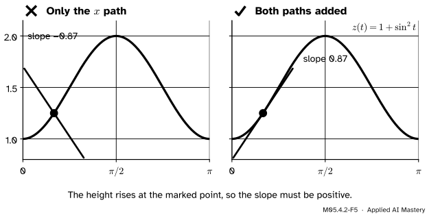
M05.4.2-F5
Wrong beside right. Keeping only the path through \(x\) gives \({-2\sin t\cos t}\), the wrong sign. Adding the path through \(y\) gives the true slope.
“\(z\) depends on \(t\) through \(x\), so \({dz/dt = \pd{z}{x}\,dx/dt}\).”
\(z\) also depends on \(t\) through \(y\), and every path counts. On the circle the \(x\) path alone gives \({(2\cos t)(-\sin t) = -2\sin t\cos t}\), the opposite of the truth: the walker climbs while that formula says she descends. Draw the tree and count the paths before you write anything.
“Cancel the \({\partial x}\): \({\pd{z}{x}\pd{x}{s}}\) is just \({\pd{z}{s}}\).”
Cancel in both terms and the chain rule would read \({\pd{z}{s} = \pd{z}{s} + \pd{z}{s}}\), which is nonsense. A partial derivative holds other variables fixed, and different partials hold different things fixed, so they are not fractions. The curly \(\partial\) is there as a warning.
“Evaluate the partial derivatives at the parameter value.”
They are evaluated at the point\({(x(t), y(t))}\). At \({t = \pi/6}\) on the circle, \({f_x = 2x}\) is \({2\cos(\pi/6) \approx 1.73}\), not \({2 \times \pi/6}\). In a network the same rule means a layer’s derivative is evaluated at the values that layer actually received.
Check yourself
Recall
1. State the chain rule for \({z = f(x, y)}\) with \({x = x(t)}\) and \({y = y(t)}\).
Show answer
\({dz/dt} = {f_x\,dx/dt + f_y\,dy/dt}\), with \(f_x\) and \(f_y\) evaluated at \({(x(t), y(t))}\); that is, \({\nabla f \cdot \vect{r}'(t)}\).
2. How do you read \({\pd{z}{s}}\) off a tree diagram?
Show answer
Multiply the branch derivatives along each path from \(z\) down to \(s\), then add the products over all such paths.
3. Why is \({\nabla f \cdot \vect{r}'(t) = 0}\) for a path inside a level set?
Show answer
On the path \(f\) stays equal to the level \(c\), so its derivative in \(t\) is 0, and by the chain rule that derivative is \({\nabla f \cdot \vect{r}'(t)}\).
4. On the circle \({(\cos t, \sin t)}\), what is the rate of change of the running bowl?
Show answer
\({2\sin t\cos t}\), which is \({\sin 2t}\); about 0.866 at \({t = \pi/6}\).
5. If \({w = uv}\), what is \({\pd{L}{u}}\) in terms of \({\pd{L}{w}}\)?
Show answer
\({\pd{L}{u} = \pd{L}{w}\,v}\): the gradient for one factor is scaled by the other factor.
Exercises
1.★ Let \({z = xy}\) with \({x = t^2}\) and \({y = e^t}\). Find \({dz/dt}\) at \({t = 1}\) by the chain rule, and check by substituting first.
Show solution
\({\pd{z}{x} = y}\) and \({\pd{z}{y} = x}\), while \({dx/dt = 2t}\) and \({dy/dt = e^t}\). At \({t = 1}\), \({x = 1}\) and \({y = e}\), so \({dz/dt} = {e \cdot 2 + 1 \cdot e} = {3e \approx 8.155}\). Substituting: \({z = t^2e^t}\), so \({z' = 2te^t + t^2e^t}\), which is \(3e\) at \({t = 1}\).
2.★★ In the running loss, let \({w = s + t}\) and \({b = s - t}\). Draw the tree and find \({\pd{L}{s}}\) and \({\pd{L}{t}}\) at \({(s, t) = (1, 0)}\).
Show solution
At \({(1, 0)}\), \({w = 1}\) and \({b = 1}\), so \({\pd{L}{w} = 15 + 5 - 23.5 = -3.5}\) and \({\pd{L}{b} = 5 + 2 - 8 = -1}\). Each parameter reaches \(L\) along two paths:
3.★★★ For any differentiable \({f(x, y)}\) with \({x = r\cos\theta}\) and \({y = r\sin\theta}\), show that \({(\pd{z}{r})^2 + r^{-2}(\pd{z}{\theta})^2 = f_x^2 + f_y^2}\), and check it with the numbers of the worked example.
Show solution
By the chain rule, \({\pd{z}{r} = f_x\cos\theta + f_y\sin\theta}\) and \({\pd{z}{\theta} = -f_x r\sin\theta + f_y r\cos\theta}\), so \({r^{-1}\pd{z}{\theta} = -f_x\sin\theta + f_y\cos\theta}\). Square both and add; the cross terms \({\pm 2f_xf_y\sin\theta\cos\theta}\) cancel, and \({\cos^2\theta + \sin^2\theta = 1}\) leaves \({f_x^2 + f_y^2}\). Check: \({5^2 + (2\sqrt3/2)^2 = 25 + 3 = 28}\), and \({f_x^2 + f_y^2 = 12 + 16 = 28}\). Both sides are the squared length of the gradient, measured in two frames.
Summary card
The rate of change adds one product per path: slope times speed.
M05.4.2-F1
Gradient dotted with velocity.
\({dz/dt} = {f_x\,x'(t) + f_y\,y'(t)} = {\nabla f \cdot \vect{r}'(t)}\).
\({\pd{z}{t_j} = \sum_i \pd{f}{x_i}\pd{x_i}{t_j}}\): multiply along paths, add the paths.
Inside a level set \({dz/dt = 0}\), so the gradient is perpendicular to it.
Sources. Each was opened and checked against this lesson on 15 November 2026.
Gilbert Strang and Edwin Herman, Calculus Volume 3 (OpenStax), Section 4.5: Theorem 4.8 (one independent variable, Equation 4.29, with the partial derivatives evaluated at \({(x, y)}\)), Theorem 4.9 (two independent variables, Equations 4.31 and 4.32), Theorem 4.10 (the generalised chain rule) and the tree diagrams of Figures 4.34 and 4.35.
Denis Auroux, MIT 18.02 Multivariable Calculus, Lecture 11: Chain rule (MIT OpenCourseWare, Fall 2007, transcript): the chain rule justified from the approximation formula by dividing by \({\Delta t}\), and the warning that cancelling the partial derivatives gives \({\pd{f}{u} = \pd{f}{u} + \pd{f}{u}}\).
Marc Peter Deisenroth, A. Aldo Faisal and Cheng Soon Ong, Mathematics for Machine Learning, Section 5.2.2: the chain rule for one parameter (Equation 5.49) and for two (Equations 5.51 to 5.53), written as a matrix product.