Seeing a function of many inputs: slices along lines and planes
A function of a thousand inputs cannot be drawn, but its values along a line are an ordinary curve and its values on a plane are a contour map. Build such slices by hand, use them as deep learning’s loss-landscape pictures do, and see what they can hide.
M05.1.3L2 Intermediate25 minIn review (what this means)
The maths and code on this page are checked by automated tests on every change, but an independent reader has not signed it off yet. Spot a mistake or a confusing step? Tell us.
Write the slice of a function along the line through a point in a direction, g(t) = f(a + t u), and compute it by hand for a quadratic.
Write the slice of a function on a plane through a point as a function of two variables, and read its contour map.
Explain the one-dimensional and two-dimensional loss-landscape pictures of deep learning as slices.
Show with a ten-input example why slices along random directions can hide a direction that curves down.
The question
Papers on deep learning are full of pictures of loss landscapes: smooth valleys, chaotic mountain ranges, wide flat basins. Yet the loss of even a small network is a function of tens of thousands of weights, and its graph would need one more dimension than that. What exactly do those pictures show, and what can they not show?
From the last lesson
1. What are the level sets of \({x^2 + y^2 + z^2}\)?
Show answer
For \({c > 0}\), spheres of radius \(\sqrt{c}\) round the origin; the origin alone for \({c = 0}\); nothing for \({c < 0}\).
2. Which score \(z\) gives a logistic probability of 0.9?
Show answer
\({z = \ln(0.9 / 0.1)}\), which is \({\ln 9 \approx 2.197}\).
Intuition
You cannot see all of a function of many inputs at once, but you can walk through it. Stand at a point \(\vect{a}\), pick a direction \(\vect{u}\), and walk along the straight line, writing down the value of the function as you go. The record is a function of one number, the distance walked: an ordinary curve that you can plot. That curve is a slice of the function.
M05.1.3-F1
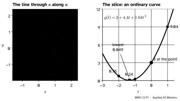
A slice. Walking along the orange line through \({\vect{a} = (1, 1)}\) in the direction \({\vect{u} = (0.6, 0.8)}\) and recording the bowl’s height gives the parabola on the right. Its lowest point, 0.049, is not the bowl’s lowest point, 0: the line misses the star.
The same walk works whether the function has two inputs or a million: a line is always one-dimensional. A plane through the point, spanned by two directions, gives a function of two numbers, which we can draw as a contour map.
Build it up
Step 1. The line. The points \({\vect{a} + t\,\vect{u}}\), for every real \(t\), form the line through \(\vect{a}\) in the direction \(\vect{u}\). When \(\vect{u}\) is a unit vector, \({\norm{\vect{u}} = 1}\), the number \(t\) is the signed distance walked from \(\vect{a}\). The direction \({(3, 4)/5 = (0.6, 0.8)}\) has length \({\sqrt{0.36 + 0.64} = 1}\).
Step 2. The slice. Feed the points of the line to \(f\): \({g(t) = f(\vect{a} + t\,\vect{u})}\). This is a composition, the line from \(\R\) to \(\R^n\) followed by \(f\) from \(\R^n\) to \(\R\), so \(g\) goes from \(\R\) to \(\R\), as in lesson M05.1.1.
Step 3. The bowl, by hand. With \({\vect{a} = (1, 1)}\) and \({\vect{u} = (0.6, 0.8)}\) the point at \(t\) is \({(1 + 0.6t,\; 1 + 0.8t)}\). Put it into \({f(x, y) = x^2 + 2y^2}\) and expand each square:
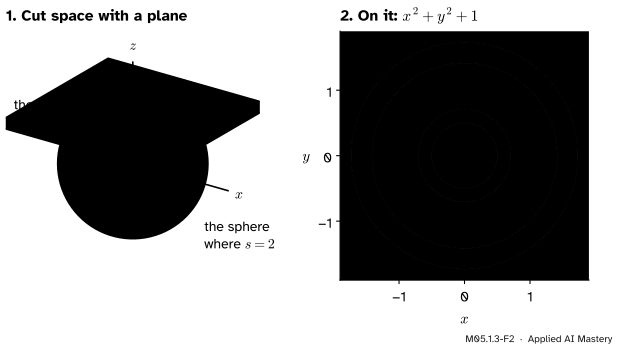
Step 4. A plane. Pick two directions \(\vect{u}\) and \(\vect{v}\) and set \({h(\alpha, \beta) = f(\vect{a} + \alpha\vect{u} + \beta\vect{v})}\). Now two numbers go in and one comes out, so \(h\) has a contour map. Take \({s(x, y, z) = x^2 + y^2 + z^2}\), the point \({(0, 0, 1)}\) and the directions of the \(x\) and \(y\) axes. The plane is \({z = 1}\), and on it \({h(\alpha, \beta) = \alpha^2 + \beta^2 + 1}\).
M05.1.3-F2
A plane slice. On the plane \({z = 1}\) the function \({x^2 + y^2 + z^2}\) becomes \({x^2 + y^2 + 1}\), a function of two inputs. Its level 2 is the circle where the plane cuts the sphere \({s = 2}\).
Step 5. Levels of a slice are cuts of levels. On the plane, \({h = 2}\) means \({\alpha^2 + \beta^2 = 1}\): a circle of radius 1. In space it is where the plane meets the sphere of radius \(\sqrt{2}\). A plane slice shows the level sets of \(f\) as the plane cuts them.
The formal statement
NoteDefinition: slices along a line and on a plane
Let \({f : \R^n \to \R}\), let \(\vect{a}\) be a point and let \(\vect{u}\), \(\vect{v}\) be directions in \(\R^n\). The slice of \(f\) along the line through \(\vect{a}\) in the direction \(\vect{u}\) is the function of one variable
\[
g(t) = f(\vect{a} + t\,\vect{u}) .
\]
The slice of \(f\) on the plane through \(\vect{a}\) spanned by \(\vect{u}\) and \(\vect{v}\) is the function of two variables
Freezing all but one input, as in M04.10.1, is the special case where \(\vect{u}\) is a coordinate direction \(\vect{e}_i\). Three facts about slices are used again and again.
The slice passes through the value at the point.\({g(0) = f(\vect{a})}\) and \({h(0, 0) = f(\vect{a})}\).
Its slope and curvature at 0 describe \(f\) at \(\vect{a}\) in the direction \(\vect{u}\). For the bowl, \({g'(t) = 4.4 + 3.28t}\), so \({g'(0) = 4.4}\): walking from \((1, 1)\) along \(\vect{u}\), the height rises 4.4 per unit of distance at first. That number is the directional derivative of M05.3.1. And \({g''(0) = 3.28}\) measures how the slope changes, the curvature of M05.5.2.
The curvature of a slice is an average of curvatures. Suppose that \({f(\vect{x}) = \lambda_1 x_1^2 + \dots + \lambda_n x_n^2}\), a sum of squares with weights. Along a unit vector \(\vect{u}\) from the origin,
Call the bracket \(k\), the slice’s curvature. Strictly, the second derivative is \({g''(0) = 2k}\), and each \(\lambda_i\) is likewise half the second derivative of \(f\) along axis \(i\); the common factor 2 changes nothing below, so we drop it. The weights \({u_i^2}\) are not negative and add up to \({\norm{\vect{u}}^2 = 1}\), so \(k\) is a weighted average of the \(\lambda_i\). A direction picks up each \(\lambda_i\) in proportion to how much it points along axis \(i\). (For the bowl, \({\lambda = (1, 2)}\) and \({k = 0.36 + 2 \cdot 0.64 = 1.64}\), half of \({g''(0) = 3.28}\).)
Go deeper: why a random direction gives each axis about 1/n of the weight
For a random unit vector drawn evenly from all directions, no axis is special, so the \(n\) weights \({u_1^2, \dots, u_n^2}\) have the same average. They add up to 1 for every \(\vect{u}\), so their averages add up to 1 too, and each average is \({1/n}\). The average curvature of a random slice is therefore \({(\lambda_1 + \dots + \lambda_n)/n}\), the mean of all the curvatures. Li and colleagues make the same point for real networks: with random Gaussian directions the curvatures of a plotted slice are weighted averages of those of the full loss, so a slice can look like a bowl whenever the upward curvatures dominate.
Worked example
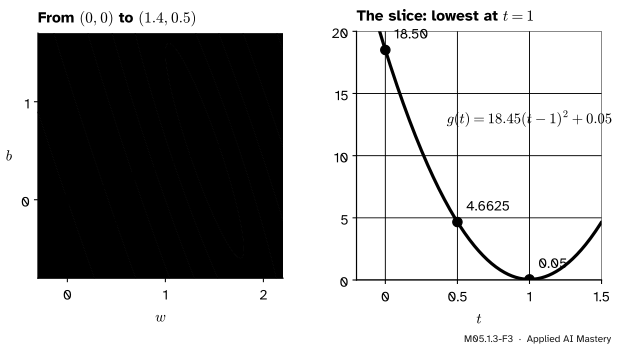
The running loss on the straight line from the origin to its minimum. Goodfellow, Vinyals and Saxe drew the loss of a network along the straight line from its starting weights to the trained ones. Do the same for \({L(w, b)}\), from \({(0, 0)}\) to the least-squares point \({(1.4, 0.5)}\). Here the direction is \({\vect{d} = (1.4, 0.5)}\), not a unit vector, so that \({t = 0}\) is the start and \({t = 1}\) the end.
The second line follows by expanding \({18.45(t^2 - 2t + 1)}\), which is \({18.45t^2 - 36.9t + 18.45}\), and adding 0.05. So \({g(0) = 18.5}\), \({g(0.5) = 4.6625}\) and \({g(1) = 0.05}\), and the slice falls steadily all the way to the minimum: no bump, no plateau on this line.
M05.1.3-F3
The worked example as a trace. The straight path from the origin to the minimum on the loss map (left) and the loss recorded along it (right): a parabola with its bottom at the end of the path.
Code
First the two slices of the worked examples, checked against the formulas.
import numpy as npbowl =lambda p: p[0]**2+2* p[1]**2loss =lambda p: 7.5* p[0]**2+5* p[0] * p[1] + p[1]**2-23.5* p[0] -8* p[1] +18.5def slice_along(f, a, u):"""The slice g(t) = f(a + t u), as a function of one variable.""" a, u = np.asarray(a, dtype=float), np.asarray(u, dtype=float)returnlambda t: f(a + t * u)g = slice_along(bowl, [1, 1], [0.6, 0.8])ell = slice_along(loss, [0, 0], [1.4, 0.5])ts = np.linspace(-3, 2, 11)print([round(float(g(t)), 4) for t in (-2, -1, 0, 1)])print([round(float(ell(t)), 4) for t in (0, 0.5, 1)])
[0.76, 0.24, 3.0, 9.04]
[18.5, 4.6625, 0.05]
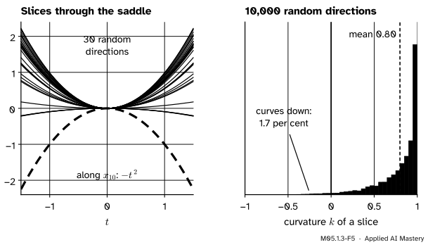
Now a function of ten inputs, the ten-input saddle\({f(\vect{x}) = x_1^2 + \dots + x_9^2 - x_{10}^2}\): nine directions curve up and one curves down, so the origin is a saddle. Slice it along 10,000 random unit directions. Each slice is \({k\,t^2}\), and three values of \(g\) give its curvature exactly: \({k = (g(1) + g(-1) - 2g(0))/2}\).
lam = np.array([1.0] *9+ [-1.0])f10 =lambda X: (lam * X**2).sum(axis=-1) # works on one point or on a stack of pointsrng = np.random.default_rng(0)U = rng.normal(size=(10_000, 10))U /= np.linalg.norm(U, axis=1, keepdims=True) # 10,000 random unit directions, as rowsk = (f10(U) + f10(-U) -2* f10(np.zeros(10))) /2print(f"mean curvature {k.mean():.3f}, curving down: {(k <0).mean():.2%}")print("along x10 alone:", f10(np.eye(10)[9]))
mean curvature 0.799, curving down: 1.67%
along x10 alone: -1.0
The mean curvature is close to \({(9 - 1)/10 = 0.8}\), as the deeper block predicts, and only 1.67 per cent of these 10,000 directions curve down. That is a seeded estimate: the exact share of all directions is 1.50 per cent, which follows from the known distribution of \(u_{10}^2\). A slice curves down only when \({u_{10}^2 > 1/2}\), when the direction points mostly along the one axis that curves down.
M05.1.3-F5
The ten-input saddle sliced along random directions. Almost every slice is a bowl; the one direction that curves down is rarely found by chance.
Explore
M05.1-X1
Level-set explorer
Choose a function and slide the level: its level set is drawn thick among its neighbours. Drag the point, or turn the line with the angle slider, and watch the slice on the right: where the line crosses the highlighted level, the slice crosses the level’s height.
Try the running bowl at \({(1, 1)}\) with the angle at 53.1°, the direction \({(0.6, 0.8)}\), and compare the slice with the anchor figure. Then turn the line until it passes through the star: only then does the slice reach the true minimum. On the saddle, turn the line through the origin from the \(x\) axis to the \(y\) axis and watch the slice change from a valley to a ridge.
Pitfalls
M05.1.3-F4
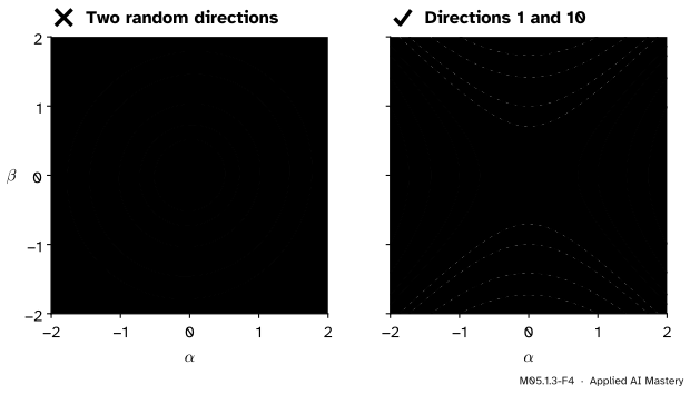
Wrong beside right. The same function of ten inputs, sliced on two planes through the origin. On a plane through two random directions it looks like a bowl; on the plane of the first and tenth axes it is plainly a saddle.
“The landscape picture shows the loss looks like a bowl, so it is a bowl.”
A slice shows the function on one line or plane only. On a random plane the curvatures are averaged, so a few directions that curve down are drowned out by many that curve up. The converse is safe: if a slice curves down somewhere, the full function does too, because that slice is part of it.
“The lowest point of the slice is the lowest point of the function.”
It is the lowest point on that line. The bowl’s slice through \((1, 1)\) along \({(0.6, 0.8)}\) bottoms out at 0.049, at \({t \approx -1.34}\), while the bowl itself reaches 0 at the origin, off the line. Only a line through the minimum, like the worked example’s, can show it.
“The width of a valley in the picture is a property of the loss.”
It depends on the length of the direction. Along \({2\vect{u}}\) the bowl’s slice is \({3 + 8.8t + 6.56t^2}\): the same values, reached twice as fast in \(t\), so the valley looks twice as narrow. This is why Li and colleagues scale each random direction to the size of the weights it perturbs before comparing pictures of different networks.
Check yourself
Recall
1. Write the slice of \(f\) along the line through \(\vect{a}\) in the direction \(\vect{u}\).
Show answer
\({g(t) = f(\vect{a} + t\,\vect{u})}\), a function of the one number \(t\).
2. What is \({g(0)}\), and what does \(t\) measure when \(\vect{u}\) is a unit vector?
Show answer
\({g(0) = f(\vect{a})}\). With \({\norm{\vect{u}} = 1}\), \(t\) is the signed distance from \(\vect{a}\) along the line.
3. What kind of picture does a slice on a plane give, and why?
Show answer
A contour map, because \({h(\alpha, \beta)}\) is a function of two numbers.
4. For \({f(\vect{x}) = \lambda_1 x_1^2 + \dots + \lambda_n x_n^2}\), what is the curvature of the slice along a unit vector \(\vect{u}\) from the origin?
Show answer
\({k = \lambda_1 u_1^2 + \dots + \lambda_n u_n^2}\), a weighted average of the \(\lambda_i\) with weights \(u_i^2\) that add up to 1.
5. Why can a two-dimensional loss-landscape picture look like a bowl when the loss has a saddle?
Show answer
Each random direction mixes all the curvatures, and when the upward ones dominate the average is positive; the few directions that curve down are almost never picked by chance.
Exercises
1.★ Find the slice of the running bowl along the \(x\) axis from \({\vect{a} = (1, 1)}\), that is with \({\vect{u} = (1, 0)}\), and compare it with M04.10.1.
Show solution
The points are \({(1 + t, 1)}\), so \({g(t) = (1 + t)^2 + 2 = 3 + 2t + t^2}\). In the variable \({x = 1 + t}\) this is \({x^2 + 2}\), the slice through \({y = 1}\) of M04.10.1, shifted so that \({t = 0}\) is the point \((1, 1)\).
2.★★ Find the slice of the saddle \({x^2 - y^2}\) along the line through the origin in the direction \({(\cos\theta, \sin\theta)}\). For which angles does it curve up, down, or not at all?
Show solution
The points are \({(t\cos\theta,\; t\sin\theta)}\), so
by the double-angle formula. It curves up when \({\cos 2\theta > 0}\) (within 45° of the \(x\) axis), down when \({\cos 2\theta < 0}\) (within 45° of the \(y\) axis), and is flat, \({g = 0}\), along the diagonals \({\theta = \pm 45°}\), which are the saddle’s level 0.
3.★★★ For the ten-input saddle, show that the slice along a unit vector \(\vect{u}\) from the origin curves down exactly when \({u_{10}^2 > 1/2}\), and find the plane slice on the plane of \(\vect{e}_1\) and \(\vect{e}_{10}\).
Show solution
The curvature is \({k = u_1^2 + \dots + u_9^2 - u_{10}^2}\). Since the squares add up to 1, \({u_1^2 + \dots + u_9^2 = 1 - u_{10}^2}\), so
which is negative exactly when \({u_{10}^2 > 1/2}\). On the plane, the point \({\alpha\vect{e}_1 + \beta\vect{e}_{10}}\) has \({x_1 = \alpha}\), \({x_{10} = \beta}\) and every other entry 0, so \({h(\alpha, \beta) = \alpha^2 - \beta^2}\): the running saddle.
Summary card
Walk a line through \(f\) and record its height: a function of any number of inputs becomes a curve.
M05.1.3-F1
A line in, a curve out.
Line slice:\({g(t) = f(\vect{a} + t\,\vect{u})}\), with \({g(0) = f(\vect{a})}\).
Bowl: from \((1, 1)\) along \({(0.6, 0.8)}\), \({g(t) = 3 + 4.4t + 1.64t^2}\).
Caution: a slice averages curvatures, and its minimum is only the minimum on that line.
Sources and next steps
Sources. Each was opened and checked against this lesson on 15 November 2026.
Hao Li, Zheng Xu, Gavin Taylor, Christoph Studer and Tom Goldstein, Visualizing the Loss Landscape of Neural Nets, NeurIPS 2018. Section 3 describes 1D linear interpolation and the plots \({f(\alpha) = L(\theta^* + \alpha\delta)}\) and \({f(\alpha, \beta) = L(\theta^* + \alpha\delta + \beta\eta)}\) (equation 1); Section 4 scales each random direction filter by filter to the norm of the weights; Section 6, “A note of caution”, states that the curvatures of a plot along random Gaussian directions are weighted averages of the full curvatures, so apparent convexity does not prove convexity, while non-convexity in the plot does imply it.
Gilbert Strang and Edwin Herman, Calculus Volume 3 (OpenStax), Section 4.1: vertical traces, the slices with one input held fixed.
Next.M05.1.4 Limits and continuity uses slices along every line into a point, and finds that even all of them together are not enough. Module M05.3 turns the slope \({g'(0)}\) into the directional derivative.