Of all directions, the gradient climbs fastest and minus the gradient falls fastest, in any number of dimensions: a two-line proof with the Cauchy-Schwarz inequality. The same arrow crosses every level set at a right angle and grows where contours crowd.
M05.3.2L2 Intermediate25 minIn review (what this means)
The maths and code on this page are checked by automated tests on every change, but an independent reader has not signed it off yet. Spot a mistake or a confusing step? Tell us.
Prove with the Cauchy-Schwarz inequality that the slope in any unit direction lies between minus and plus the length of the gradient.
Find the directions of steepest ascent, steepest descent and zero slope at a point of a function of n inputs.
Show that the gradient is perpendicular to every curve inside a level set, and relate the spacing of contours to the gradient’s length.
Explain why minus the gradient can point across a narrow valley, and even away from the minimum.
Confirm the steepest direction numerically by scanning many unit directions in three dimensions.
The question
A model with a million weights can step in infinitely many directions, and the last lesson gave the slope of the loss along any one of them. Which direction lowers the loss fastest, and how fast? In two dimensions you could turn a compass and look (M04.10.3). In a million dimensions there is no compass to turn, so the answer has to come from a proof.
From the last lesson
1. What is the slope of the running bowl \({x^2 + 2y^2}\) at \({(1, 1)}\) in the direction \({(0.6, 0.8)}\)?
Show answer
\({\nabla f = (2, 4)}\), so the slope is \({2 \times 0.6 + 4 \times 0.8 = 4.4}\).
2. Why must the direction in \({D_{\vect{u}} f}\) have length 1?
Show answer
So that the step \(s\) measures distance. A direction \(k\) units long multiplies the slope by \(k\).
Intuition
The slope in a unit direction \(\vect{u}\) is \({\nabla f\T\vect{u}}\), the shadow of the gradient on \(\vect{u}\). A fixed arrow casts its longest shadow on a line that points along the arrow itself. So the steepest way up is along the gradient, the steepest way down is straight against it, and the directions at right angles to it are level.
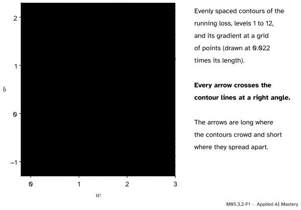
M05.3.2-F1
Evenly spaced contours of the running loss and its gradient at a grid of points. Every arrow crosses the contour lines at a right angle, and its length tells how tightly they are packed.
The picture shows two more facts that this lesson proves. Each arrow crosses the contour lines at a right angle, because walking along a contour line keeps \(f\) level. And the arrows are long exactly where evenly spaced contours crowd, because a steep slope reaches the next level in a short distance.
Build it up
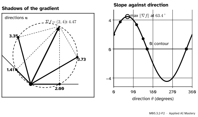
Step 1. The slope as a shadow. At \({(1, 1)}\) on the bowl the gradient is \({(2, 4)}\). Drop a perpendicular from its tip onto the line of each direction: the foot of that perpendicular marks the slope. Along \({0^\circ}\) the shadow is 2, along \({30^\circ}\) it is 3.73, along \({105^\circ}\) it is 3.35, along \({135^\circ}\) it is 1.41.
M05.3.2-F2
Every shadow’s foot sees the gradient at a right angle, so all the feet lie on the circle whose diameter is the gradient (Thales). The longest shadow is the diameter itself.
Step 2. The shadow through an angle. For a unit \(\vect{u}\), the dot product is \({\nabla f\T\vect{u}} = {\norm{\nabla f}\norm{\vect{u}}\cos\theta} = {\norm{\nabla f}\cos\theta}\), where \(\theta\) is the angle between the gradient and \(\vect{u}\) (M02.3.3). As \(\vect{u}\) turns, the slope traces a cosine of height \({\norm{\nabla f}}\), the wave on the right.
Step 3. Any number of dimensions. The angle between two vectors is defined in \(\R^n\) by the same formula, and two vectors always span a flat plane. Whatever \(n\) is, the gradient and the chosen direction sit in one plane, and the picture of Step 1 is the picture in that plane.
The formal statement
NoteResult: steepest ascent
Let \(f\) be differentiable at \(\vect{a}\) with gradient \({\vect{g}} = {\nabla f(\vect{a}) \neq \vect{0}}\). For every unit vector \(\vect{u}\),
The largest slope is reached only at \({\vect{u} = \vect{g}/\norm{\vect{g}}}\), the direction of steepest ascent; the smallest only at \({\vect{u} = -\vect{g}/\norm{\vect{g}}}\), the direction of steepest descent. The slope is 0 exactly for the \(\vect{u}\) perpendicular to \(\vect{g}\). If \({\vect{g} = \vect{0}}\), every slope is 0.
Proof. By lesson 1, \({D_{\vect{u}} f(\vect{a})} = {\vect{g}\T\vect{u}}\). The Cauchy-Schwarz inequality (M02.3.3) gives
which is the double inequality. Equality in Cauchy-Schwarz holds only when one vector is a multiple of the other, so \({\vect{u} = k\vect{g}}\); a unit \(\vect{u}\) then has \({k = \pm 1/\norm{\vect{g}}}\). The plus sign gives \({\vect{g}\T\vect{g}/\norm{\vect{g}}} = {\norm{\vect{g}}}\), the top; the minus sign gives \({-\norm{\vect{g}}}\), the bottom. A dot product is 0 exactly when the vectors are perpendicular. \(\square\)
In \({\R^n}\) the level directions are not two arrows but all the directions perpendicular to \(\vect{g}\): a flat set of dimension \({n - 1}\). The next result says what they are.
NoteResult: the gradient is perpendicular to level sets
Let \(f\) be differentiable at \(\vect{a}\), let \({c = f(\vect{a})}\), and let \({\vect{r}(t)}\) be a curve with \({\vect{r}(0) = \vect{a}}\) that stays in the level set, \({f(\vect{r}(t)) = c}\), and has a velocity \({\vect{r}'(0)}\). Then \({\nabla f(\vect{a})\T\vect{r}'(0) = 0}\).
Proof. Write \({\vect{h}(t) = \vect{r}(t) - \vect{a}}\), which shrinks to \(\vect{0}\) as \({t \to 0}\). Differentiability at \(\vect{a}\) gives, with the remainder \(r\) of lesson 1,
The left side is 0 because the curve stays at level \(c\). Divide by \({t \neq 0}\). The first term becomes \({\nabla f(\vect{a})\T(\vect{h}(t)/t)}\), and \({\vect{h}(t)/t \to \vect{r}'(0)}\). In the second, where \({\vect{h}(t) \neq \vect{0}}\) write \({r(\vect{h})/t} = {\big(r(\vect{h})/\norm{\vect{h}}\big)\big(\norm{\vect{h}}/t\big)}\): the first factor tends to 0 and the second stays bounded, since its size tends to \({\norm{\vect{r}'(0)}}\). Where \({\vect{h}(t) = \vect{0}}\) the remainder is 0. So in the limit \({0 = \nabla f(\vect{a})\T\vect{r}'(0)}\). \(\square\)
A curve inside the level set can leave \(\vect{a}\) in any direction tangent to the set, so the gradient is perpendicular to the whole tangent direction of the level set. M05.4.2 reaches the same result again with the chain rule.
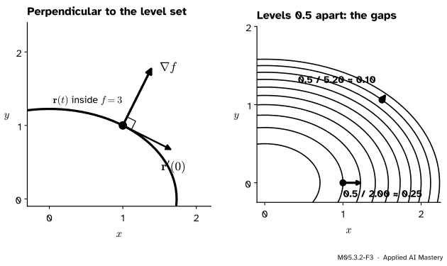
Spacing of contours. Step from \(\vect{a}\) a short distance \(s\) along \({\vect{g}/\norm{\vect{g}}}\). By lesson 1, \(f\) rises by about \({\norm{\vect{g}}\,s}\). To rise by \(\delta\) to the next level takes
\[
s \approx \frac{\delta}{\norm{\nabla f(\vect{a})}} .
\]
Evenly spaced contours sit close where the gradient is long and far apart where it is short.
M05.3.2-F3
Left: the velocity of a curve inside a level set is at right angles to the gradient. Right: the gap to the next level is about the level step divided by \({\norm{\nabla f}}\), so it shrinks where the gradient grows.
Go deeper: does every tangent direction come from a curve in the level set?
The result above needs a curve in the level set to exist. When \({\nabla f(\vect{a}) \neq \vect{0}}\) and the partial derivatives are continuous near \(\vect{a}\), the implicit function theorem guarantees that near \(\vect{a}\) the level set is a smooth curve (in the plane), surface (in space) or hypersurface (in \(\R^n\)), with a curve through \(\vect{a}\) in every direction perpendicular to the gradient. We state it without proof. At a point where the gradient is \(\vect{0}\) the level set can look like anything: for the saddle \({x^2 - y^2}\) the level set through the origin is two crossing lines, which have no single tangent direction there.
Worked example
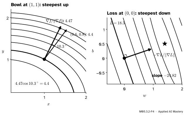
The bowl at \({(1, 1)}\). The gradient is \({(2, 4)}\) with length \({\sqrt{4 + 16} = \sqrt{20} \approx 4.472}\). Steepest ascent is \({(2, 4)/\sqrt{20}} = {(1, 2)/\sqrt{5}} \approx {(0.447, 0.894)}\), with slope 4.472; steepest descent is the opposite unit vector, with slope \(-4.472\). The level directions are \({\pm(2, -1)/\sqrt{5}}\), since \({2 \times 2 + 4 \times (-1) = 0}\). The direction \({(0.6, 0.8)}\) of lesson 1 had slope 4.4, so the angle \(\theta\) between it and the gradient satisfies
The running loss at \({(0, 0)}\). The gradient \({(-23.5, -8)}\) has length \({\sqrt{552.25 + 64}} = {\sqrt{616.25}} \approx {24.824}\). Steepest descent is \({(23.5, 8)/24.824 \approx (0.947, 0.322)}\), with slope \(-24.824\). The direction towards the lowest point in lesson 1 had slope \(-24.822\): only about \({0.85^\circ}\) away from the steepest.
M05.3.2-F4
The worked example as a trace. On the bowl the unit gradient beats \({(0.6, 0.8)}\) by the factor \({\cos 10.3^\circ}\); on the loss the steepest way down from the origin meets its contour at a right angle.
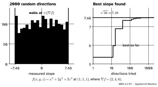
Three inputs. For \({f = x^2 + 2y^2 + 3z^2}\) at \({(1, 1, 1)}\), \({\nabla f = (2, 4, 6)}\) and the steepest slope is \({\sqrt{4 + 16 + 36}} = {\sqrt{56}} \approx {7.483}\). The level directions form a plane: every \(\vect{u}\) with \({2u_1 + 4u_2 + 6u_3 = 0}\), such as \({(2, -1, 0)}\) and \({(3, 0, -1)}\) after normalising.
Code
A brute-force test of the theorem in three dimensions: two thousand random unit directions, each slope measured by a central difference, and the best of them compared with \({\nabla f}\).
import numpy as npf =lambda p: p[..., 0] **2+2* p[..., 1] **2+3* p[..., 2] **2a = np.array([1.0, 1.0, 1.0])grad = np.array([2.0, 4.0, 6.0])rng = np.random.default_rng(0)u = rng.normal(size=(2000, 3))u /= np.linalg.norm(u, axis=1, keepdims=True) # random points on the unit sphereh =1e-5slopes = (f(a + h * u) - f(a - h * u)) / (2* h) # measured, not from the formulabest = np.argmax(slopes)angle = np.degrees(np.arccos(u[best] @ grad / np.linalg.norm(grad)))print("largest measured slope:", round(slopes.max(), 4), " |grad f| =", round(np.linalg.norm(grad), 4))print("smallest measured slope:", round(slopes.min(), 4))print("angle between the best direction and grad f:", round(angle, 2), "degrees")
largest measured slope: 7.4824   |grad f| = 7.4833
smallest measured slope: -7.4753
angle between the best direction and grad f: 0.92 degrees
No direction beats \({\sqrt{56} \approx 7.483}\), and the best one found lies within about a degree of the gradient; with more directions it creeps closer.
M05.3.2-F5
Measured slopes along random directions never pass \({\pm\norm{\nabla f}}\), and the best so far approaches \({\sqrt{56}}\) from below as more directions are tried.
Two more checks: Cauchy-Schwarz in ten dimensions at random points and directions, and the spacing rule on the bowl from \({(1, 0)}\), where the next contour, \({f = 1.5}\), crosses the axis at \({x = \sqrt{1.5}}\).
for _ inrange(1000): g, v = rng.normal(size=10), rng.normal(size=10) v /= np.linalg.norm(v)assertabs(g @ v) <= np.linalg.norm(g) +1e-12# slope never beyond |g|gap_true = np.sqrt(1.5) -1.0gap_estimate =0.5/ np.linalg.norm([2.0, 0.0])print(f"gap to the next level: true {gap_true:.4f}, estimate {gap_estimate:.4f}")
gap to the next level: true 0.2247, estimate 0.2500
Explore
The direction dial in lesson 3 draws the slope against the angle beside the contour map. Press Along the gradient and the marker sits on the peak of the cosine; press Along the contour and it sits on a zero. Drag the point towards the edge of the loss’s valley and watch the peak grow as the contours crowd.
Pitfalls
M05.3.2-F6
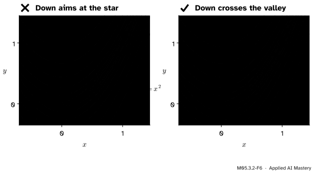
Wrong beside right on the running valley at \({(0, 0.5)}\). The steepest way down drops almost vertically into the valley, \({115^\circ}\) away from the direction of the lowest point.
“Minus the gradient points at the minimum.”
It points straight downhill where you stand, at right angles to the contour. On the running valley \({(1 - x)^2 + 100(y - x^2)^2}\) the two partial derivatives are
which at \({(0, 0.5)}\) give \({\nabla f = (-2, 100)}\). The way down, \({(2, -100)}\), is almost straight down, while the minimum \({(1, 1)}\) lies up and to the right: \({115^\circ}\) apart. A short step downhill even moves away from the minimum. Gradient descent first falls into the valley floor, then crawls along it, and in a narrow valley it bounces from wall to wall in a zigzag (M03.8.4).
“A zero gradient means the bottom.”
A zero gradient means every slope is 0, to first order, in every direction. The saddle \({x^2 - y^2}\) has gradient \({(2x, -2y) = (0, 0)}\) at the origin, yet it rises along the \(x\) axis and falls along the \(y\) axis. Telling a minimum from a saddle takes second derivatives (M05.5).
“Crowded contours mean large values.”
Crowding means a steep slope, not a high value. Add 1000 to a loss and every value changes, yet no contour line moves and no gap changes. Double the loss and its values double while every gap between levels \(\delta\) apart halves, because the gradient doubles. The gaps measure \({\norm{\nabla L}}\), not \(L\).
Check yourself
Recall
1. Between which two numbers does \({D_{\vect{u}} f(\vect{a})}\) lie, and which inequality says so?
Show answer
Between \({-\norm{\nabla f(\vect{a})}}\) and \({\norm{\nabla f(\vect{a})}}\), by the Cauchy-Schwarz inequality.
2. What is the direction of steepest descent, and what is the slope along it?
Show answer
\({-\nabla f/\norm{\nabla f}}\), with slope \({-\norm{\nabla f}}\).
3. How does the gradient sit relative to a level set through the point?
Show answer
It is perpendicular to it: perpendicular to the velocity of every curve that stays in the level set.
4. Evenly spaced contours are close together in one place. What does that say about the gradient there?
Show answer
It is long. The gap between levels \(\delta\) apart is about \({\delta/\norm{\nabla f}}\).
5. In \(\R^n\), which directions have slope 0 at a point where \({\nabla f \neq \vect{0}}\)?
Show answer
All unit vectors perpendicular to the gradient: a set of dimension \({n - 1}\), the tangent directions of the level set.
Exercises
1.★ For the running bowl at \({(-1, 0.5)}\), find the directions of steepest ascent and descent, the steepest slope, and the level directions.
Show solution
\({\nabla f = (2x, 4y) = (-2, 2)}\), of length \({\sqrt{8} \approx 2.83}\). Steepest ascent is \({(-1, 1)/\sqrt{2}}\) with slope \({\sqrt{8}}\), steepest descent \({(1, -1)/\sqrt{2}}\) with slope \({-\sqrt{8}}\), and the level directions are \({\pm(1, 1)/\sqrt{2}}\), since \({-2 + 2 = 0}\).
2.★★ For \({f = x^2 + 2y^2 + 3z^2}\) at \({(1, 1, 1)}\), find the slope along \({(1, 1, 1)/\sqrt{3}}\) and the angle between that direction and the gradient.
Show solution
The slope is \({(2 + 4 + 6)/\sqrt{3}} = {12/\sqrt{3}} \approx {6.93}\). The steepest slope is \({\sqrt{56} \approx 7.483}\), so
and \({\theta \approx 22.2^\circ}\). The diagonal is a good direction, but not the best.
3.★★★ On the bowl, step from \({(1, 1)}\) along the steepest-ascent direction \({(1, 2)/\sqrt{5}}\). Find the exact distance \(s\) at which \(f\) reaches 3.5 and compare it with the estimate \({\delta/\norm{\nabla f}}\).
Show solution
On the line, \({x = 1 + s/\sqrt{5}}\) and \({y = 1 + 2s/\sqrt{5}}\), so
\({\nabla f\T\vect{r}'(0) = 0}\) for every curve in a level set.
Gap between levels \(\delta\) apart: about \({\delta/\norm{\nabla f}}\).
Bowl at \({(1, 1)}\): 4.472. Loss at \({(0, 0)}\): \(-24.824\) along \({(0.947, 0.322)}\).
Sources and next steps
Sources. Each was opened and checked against this lesson on 15 November 2026.
Gilbert Strang and Edwin Herman, Calculus Volume 3 (OpenStax), Section 4.6: Theorem 4.13 (the directional derivative is largest along the gradient, with value its length, smallest straight against it, and 0 in every direction when the gradient is zero) and Theorem 4.14 (the gradient is normal to the level curve).
Denis Auroux, MIT OpenCourseWare 18.02SC Multivariable Calculus, Session 36: Proof, whose reading proves that the gradient is perpendicular to every curve on a level surface through the point, and Session 38: Directional derivatives, whose reading writes the slope as the gradient’s length times \({\cos\theta}\) and concludes that it is greatest along the gradient.
Marc Peter Deisenroth, A. Aldo Faisal and Cheng Soon Ong, Mathematics for Machine Learning, Section 7.1: the gradient points in the direction of steepest ascent and is orthogonal to the contour lines, and gradient descent steps along the negative gradient (Equation 7.5, written with a transpose because the book uses row gradients).