Divergence measures how much a field flows out of a tiny square, per unit area. Derive it from the four sides of a square, read it as the trace of the Jacobian, check the divergence theorem on the unit square, and see why continuous normalising flows need it.
M05.10.3L2 Intermediate25 minIn review (what this means)
The maths and code on this page are checked by automated tests on every change, but an independent reader has not signed it off yet. Spot a mistake or a confusing step? Tell us.
Derive div F = dP/dx + dQ/dy as the limit of the net flux out of a small square divided by its area.
Compute the divergence of a field, identify it as the trace of the Jacobian, and read sources and sinks from its sign.
Check the divergence theorem in the plane by computing the flux through each side of the unit square and the double integral of the divergence.
Explain how the divergence sets the rate at which log-density changes along a flow, and estimate a trace with Hutchinson’s random-vector estimator.
The question
A continuous normalising flow turns a simple cloud of random points into realistic data by carrying every point along a learned vector field. To train it, the model must know how the density of the cloud changes as the points move: where they crowd together it rises, where they spread apart it falls. What single number, at each point of a field, says how fast things spread?
From the last lesson
1. State the fundamental theorem for gradients.
Show answer
\({\int_C \nabla f \cdot d\vect{r} = f(\text{end}) - f(\text{start})}\): the work of a gradient field is the change in its potential.
2. What is the circulation of the rotation \({(-y, x)}\) round the unit circle, and what does it show?
Show answer
\({2\pi}\). Being non-zero, it shows that the rotation is not a gradient field.
Intuition
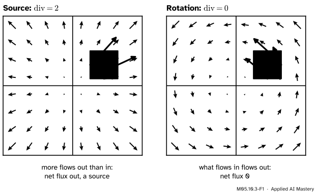
Think of the field as the velocity of a thin sheet of fluid. Draw a small square and ask how much fluid leaves it each second, minus how much enters. That net outflow is the flux out of the square. If it is positive, fluid is being created inside: a source. If negative, it is being removed: a sink.
M05.10.3-F1
The same small square in two fields. The source lets more out than in, so it creates fluid at every point. The rotation moves fluid through the square without creating any.
The divergence is that net outflow per unit area, in the limit of a tiny square. It is one number at each point: positive at a source, negative at a sink, zero where fluid only passes through.
Build it up
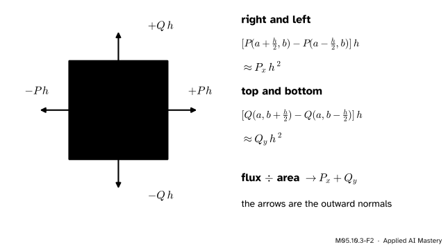
Step 1. Flux through one short side. Across a short side of length \(h\) with outward unit normal \(\vect{n}\), the fluid that crosses per second is about \({(\vect{F} \cdot \vect{n})\,h}\): only the component of the arrow across the side carries fluid over it.
Step 2. The four sides of a square. Take the square of side \(h\) centred at \({(a, b)}\). The right side has \({\vect{n} = (1, 0)}\), so \({\vect{F} \cdot \vect{n} = P}\); the left side has \({\vect{n} = (-1, 0)}\) and gives \({-P}\). Top and bottom give \({+Q}\) and \({-Q}\).
M05.10.3-F2
The flux out of a small square, side by side. Right and left together measure how much \(P\) changes across the square; top and bottom, how much \(Q\) changes.
Step 3. Pair the opposite sides. Right plus left is about \({[P(a + \tfrac{h}{2}, b) - P(a - \tfrac{h}{2}, b)]\,h}\). The bracket is the change in \(P\) over a distance \(h\) in the \(x\)-direction, about \({\pd{P}{x}\,h}\). So right plus left is about \({\pd{P}{x}\,h^2}\), and in the same way top plus bottom is about \({\pd{Q}{y}\,h^2}\).
Step 4. Divide by the area. The net flux divided by \({h^2}\) is about \({\pd{P}{x} + \pd{Q}{y}}\), and the approximation becomes exact as \({h \to 0}\).
The formal statement
NoteDefinition: divergence
For a field \({\vect{F} = (P, Q)}\) with continuous partial derivatives,
It is the trace of the Jacobian \({\mat{J}_{\vect{F}}}\) of M05.4.1, the sum of its diagonal entries. In \(\R^n\), \({\operatorname{div}\vect{F} = \sum_i \pd{F_i}{x_i} = \operatorname{tr}\mat{J}_{\vect{F}}}\), also written \({\nabla \cdot \vect{F}}\).
NoteTheorem: divergence as flux per area
If \(S_h\) is the square of side \(h\) centred at \({(a, b)}\), then
Proof. The right side runs over \({y \in [b - \tfrac{h}{2}, b + \tfrac{h}{2}]}\) at \({x = a + \tfrac{h}{2}}\), the left side at \({x = a - \tfrac{h}{2}}\). Their flux together is
For each \(y\), the mean value theorem in \(x\) writes the bracket as \({h\,\pd{P}{x}(\xi_y, y)}\) for some \({\xi_y}\) between the two sides. So the pair contributes \(h\) times the integral of \({\pd{P}{x}(\xi_y, y)}\) over an interval of length \(h\), that is \({h^2}\) times an average of \({\pd{P}{x}}\) over points inside the square. As \({h \to 0}\) those points close in on \({(a, b)}\), and because \({\pd{P}{x}}\) is continuous the average tends to \({\pd{P}{x}(a, b)}\). Top and bottom give \({\pd{Q}{y}(a, b)}\) the same way. Add the two and divide by \({h^2}\). ∎
The running fields. The source \({(x, y)}\) has divergence \({1 + 1 = 2}\) everywhere. The rotation \({(-y, x)}\) has \({0 + 0 = 0}\). The bowl’s gradient \({(2x, 4y)}\) has \({2 + 4 = 6}\): for a gradient, \({\operatorname{div}\nabla f = f_{xx} + f_{yy}}\), the trace of the Hessian, called the Laplacian. The score \({-(x, y)}\) of the standard Gaussian has divergence \({-2}\): a sink at every point.
NoteTheorem: the divergence theorem in the plane
For a region \(D\) bounded by a closed curve \(C\) with outward normal \(\vect{n}\), and \(\vect{F}\) with continuous partial derivatives on and inside \(C\),
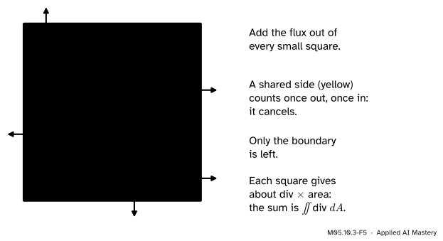
This is also called the flux form of Green’s theorem; lesson M05.10.4 proves Green’s theorem for a rectangle, and this form follows from it by applying it to \({(-Q, P)}\). The picture explains why it must hold.
M05.10.3-F5
Why the theorem holds. Every inside side is shared by two squares with opposite normals, so its flux cancels in the sum; what survives is the flux through the boundary.
In three dimensions the same argument with small cubes gives \({\iint_S \vect{F} \cdot \vect{n}\,dS = \iiint_E \operatorname{div}\vect{F}\,dV}\), with \({\operatorname{div}\vect{F} = P_x + Q_y + R_z}\): the flux out of a closed surface equals the total divergence inside.
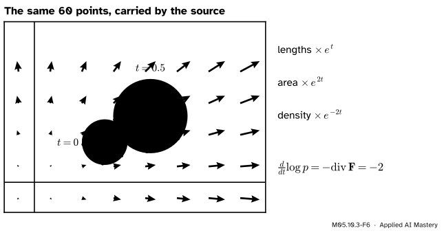
Divergence moves density. Carry a cloud of points along a field. Mass is neither made nor lost, so the density \({p(\vect{x}, t)}\) obeys the continuity equation, stated here without proof: \({\partial p/\partial t + \operatorname{div}(p\,\vect{F}) = 0}\). Follow one point along its flow line. By the chain rule its density changes at the rate
The last line uses the product rule, \({\operatorname{div}(p\vect{F}) = \nabla p \cdot \vect{F} + p\,\operatorname{div}\vect{F}}\). Dividing by \(p\) gives
The source flow carries a blob outwards. Lengths grow by \({e^t}\), so areas by \({e^{2t}}\), and the same points spread over more area: the density falls by \({e^{-2t}}\), as \({\operatorname{div} = 2}\) predicts.
Chen and colleagues proved this rule for the flows of neural ODEs, in the form \({d\log p/dt = -\operatorname{tr}(\partial \vect{f}/\partial\vect{z})}\), and it is how continuous normalising flows (M12.7) compute likelihoods: a trace instead of the determinant of M05.6.4.
Worked example
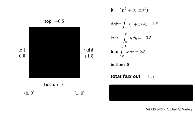
The divergence theorem on the unit square. Take the cubic field \({\vect{F} = (x^3 + y,\; xy^2)}\) on the square \({0 \le x, y \le 1}\). Its divergence is \({\pd{P}{x} + \pd{Q}{y} = 3x^2 + 2xy}\).
The flux, side by side. On the right side \({x = 1}\), \({\vect{n} = (1, 0)}\) and \({P = 1 + y}\), giving \({\int_0^1 (1 + y)\,dy = 1.5}\). On the left side \({x = 0}\), \({\vect{n} = (-1, 0)}\) and \({-P = -y}\), giving \({-0.5}\). On the top \({y = 1}\), \({Q = x}\), giving \({\int_0^1 x\,dx = 0.5}\). On the bottom \({y = 0}\), \({Q = 0}\). The total flux out is \({1.5 - 0.5 + 0.5 + 0 = 1.5}\).
M05.10.3-F3
The worked example as a trace. Four sides, four fluxes, total 1.5; and the integral of the divergence over the square is 1.5 too.
The divergence, integrated. Over the unit square, \({\iint 3x^2\,dA = 1}\) and \({\iint 2xy\,dA = 2 \cdot \tfrac12 \cdot \tfrac12 = 0.5}\), so the total is 1.5. The two sides of the theorem agree.
A small square. Now centre a square of side \(h\) at \({(1, 0.5)}\), where the divergence is \({3 + 1 = 4}\). Right minus left: the \(y\) terms cancel and
integrated over a side of length \(h\), giving \({3h^2 + h^4/4}\). Top minus bottom: \({Q = xy^2}\) and \({(0.5 + \tfrac{h}{2})^2 - (0.5 - \tfrac{h}{2})^2 = h}\), so the pair gives \({h \int x\,dx = h \cdot h \cdot 1 = h^2}\). Divided by \({h^2}\) the flux per area is \({4 + h^2/4}\): 4.25 for \({h = 1}\), 4.0625 for \({h = 0.5}\), and 4 in the limit.
Code
The flux out of a square, from scratch, with each side integrated by quad, set beside the divergence formula.
import numpy as npfrom scipy.integrate import quaddef flux_out_of_square(F, a, b, h):"""Net flux of F = (P, Q) out of the square of side h centred at (a, b).""" lo_x, hi_x, lo_y, hi_y = a - h /2, a + h /2, b - h /2, b + h /2 right = quad(lambda y: F(hi_x, y)[0], lo_y, hi_y)[0] left =-quad(lambda y: F(lo_x, y)[0], lo_y, hi_y)[0] top = quad(lambda x: F(x, hi_y)[1], lo_x, hi_x)[0] bottom =-quad(lambda x: F(x, lo_y)[1], lo_x, hi_x)[0]return right + left + top + bottomcubic =lambda x, y: (x **3+ y, x * y **2)div_cubic =lambda x, y: 3* x **2+2* x * yprint("unit square:", round(flux_out_of_square(cubic, 0.5, 0.5, 1.0), 6))for h in (1.0, 0.5, 0.1, 0.01):print(f"h = {h}: flux / area = {flux_out_of_square(cubic, 1.0, 0.5, h) / h **2:.6f}")print("div at (1, 0.5):", div_cubic(1.0, 0.5))
unit square: 1.5
h = 1.0: flux / area = 4.250000
h = 0.5: flux / area = 4.062500
h = 0.1: flux / area = 4.002500
h = 0.01: flux / area = 4.000025
div at (1, 0.5): 4.0
Hutchinson’s estimator. The trace of a large Jacobian costs one derivative pass per input, but a random vector \(\vect{e}\) with independent entries \({\pm 1}\) gives \({\E[\vect{e}\T\mat{J}\vect{e}] = \operatorname{tr}\mat{J}}\), because \({\vect{e}\T\mat{J}\vect{e} = \sum_{i,j} J_{ij}e_ie_j}\) and \({\E[e_ie_j]}\) is 1 when \({i = j}\) and 0 otherwise. Reverse mode (M05.8) computes \({\vect{e}\T\mat{J}}\) for about the cost of one evaluation.
J = np.array([[3.0, 1.0], [0.25, 1.0]]) # Jacobian of the cubic field at (1, 0.5)signs = [np.array([s1, s2]) for s1 in (1, -1) for s2 in (1, -1)]values = [e @ J @ e for e in signs]print("e^T J e over the four sign vectors:", values, " mean:", np.mean(values), " trace:", np.trace(J))rng = np.random.default_rng(0)A = rng.normal(size=(200, 200))E = rng.choice([-1.0, 1.0], size=(2000, 200))estimate = np.mean(np.einsum("ki,ij,kj->k", E, A, E))print("200 x 200: trace", round(np.trace(A), 2), " estimate from 2000 vectors", round(estimate, 2))
e^T J e over the four sign vectors: [np.float64(5.25), np.float64(2.75), np.float64(2.75), np.float64(5.25)]  mean: 4.0  trace: 4.0
200 x 200: trace 5.17  estimate from 2000 vectors -0.21
With four sign vectors the average is the trace exactly. For the random \({200 \times 200}\) matrix the estimate lands within a few standard errors of the trace; the exact digits depend on the random draw, so the check allows that spread.
Explore
M05.10-X1
Field explorer
Choose a field, drag the small square (or use its sliders) and compare the flux out of it, divided by its area, with the divergence at its centre; shrink the square to see them meet. Click the drawing, or press the drop button, to release particles that follow the arrows by small Euler steps.
Pitfalls
M05.10.3-F4
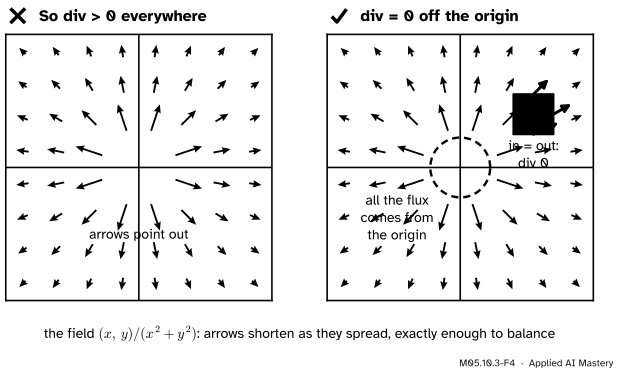
Wrong beside right. Arrows that point outwards do not make a source: this field thins out exactly as fast as it spreads, so every small square away from the origin lets out what it takes in.
“The arrows point away from the centre, so the divergence is positive.”
For \({\vect{F} = (x, y)/(x^2 + y^2)}\), \({\pd{P}{x} = (y^2 - x^2)/(x^2 + y^2)^2}\) and \({\pd{Q}{y} = (x^2 - y^2)/(x^2 + y^2)^2}\), which add to 0. All of its flux comes from the origin: round any circle centred there it is \({2\pi}\). Divergence is about how the arrows change across a small square, not which way they point.
“The divergence is the flux out of the square.”
It is flux per unit area. The source lets \({2h^2}\) out of a square of side \(h\): 8 from a square of side 2, 0.02 from a square of side 0.1. Its divergence is 2 for both. Only after dividing by the area does the number stop depending on the square.
“Zero divergence means the flow is standing still.”
The rotation has divergence 0 and moves everything. Zero divergence means the flow preserves area: a blob carried by it changes shape and position but not size. A normalising flow with zero divergence only moves density values around, never raising or lowering them, so it cannot concentrate probability where the data are dense.
Check yourself
Recall
1. Define the divergence of \({\vect{F} = (P, Q)}\) and say which matrix it is the trace of.
Show answer
\({\operatorname{div}\vect{F} = \pd{P}{x} + \pd{Q}{y}}\), the trace of the Jacobian \({\mat{J}_{\vect{F}}}\).
2. What limit defines the divergence geometrically?
Show answer
The net flux out of a small square (or any small region) divided by its area, as the square shrinks to the point.
3. Give the divergence of the source, the rotation and the bowl’s gradient field.
Show answer
2, 0 and 6.
4. State the divergence theorem in the plane.
Show answer
\({\oint_C \vect{F} \cdot \vect{n}\,ds} = {\iint_D \operatorname{div}\vect{F}\,dA}\): the flux out through the boundary equals the integral of the divergence inside.
5. Along a flow line of \(\vect{F}\), how does the log-density of the moving cloud change?
Show answer
\({d\log p/dt = -\operatorname{div}\vect{F}}\): it falls where the field spreads and rises where it converges.
Exercises
1.★ Compute the divergence of \({\vect{F} = (xy,\; y^2 - x^2)}\) and say where the field acts as a source.
Show solution
\({\pd{P}{x} = y}\) and \({\pd{Q}{y} = 2y}\), so \({\operatorname{div}\vect{F} = 3y}\). It is a source above the \(x\)-axis, a sink below it, and neither on the axis.
2.★★ Check the divergence theorem for the source \({(x, y)}\) on the unit disc.
Show solution
On the unit circle the outward normal is \({\vect{n} = (x, y)}\) itself, so \({\vect{F} \cdot \vect{n} = x^2 + y^2 = 1}\) and the flux is the circle’s length, \({2\pi}\). Inside, \({\operatorname{div}\vect{F} = 2}\), and \({\iint_D 2\,dA = 2\pi}\), twice the disc’s area. Both give \({2\pi}\).
3.★★★ For a \({2 \times 2}\) matrix \(\mat{J}\) and \({\vect{e} = (e_1, e_2)}\) with independent signs \({\pm 1}\) of equal probability, show that \({\vect{e}\T\mat{J}\vect{e}} = {\operatorname{tr}\mat{J} + e_1e_2(J_{12} + J_{21})}\). Deduce that the estimator is unbiased, find its variance, and say when a single sample is exact.
Since \({e_i^2 = 1}\), this is \({J_{11} + J_{22}} + {e_1e_2(J_{12} + J_{21})}\). The product \({e_1e_2}\) is \({\pm 1}\) with equal probability, so its mean is 0 and the estimator’s mean is \({\operatorname{tr}\mat{J}}\). Its variance is \({(J_{12} + J_{21})^2}\), since \({(e_1e_2)^2 = 1}\). One sample is exact when \({J_{12} = -J_{21}}\), that is when the off-diagonal part of \(\mat{J}\) is antisymmetric. For the cubic field at \({(1, 0.5)}\), \({J_{12} + J_{21} = 1.25}\): samples 5.25 and 2.75, mean 4.
Summary card
Divergence is the flux out of a tiny square, per unit area.
Along a flow, \({d\log p/dt} = {-\operatorname{div}\vect{F}}\); Hutchinson: \({\E[\vect{e}\T\mat{J}\vect{e}]} = {\operatorname{tr}\mat{J}}\).
Sources and next steps
Sources. Each was opened and checked against this lesson on 15 November 2026.
Gilbert Strang and Edwin Herman, Calculus Volume 3, Section 6.5 (OpenStax): divergence in the plane and in space (Equation 6.16), and its reading as a source where it is positive and a sink where it is negative. Section 6.4 gives the flux form of Green’s theorem (Theorem 6.13, Equation 6.15), and Section 6.8 the divergence theorem in space (Theorem 6.20, Equation 6.24).
Denis Auroux, MIT 18.02SC, Session 70: Normal form of Green’s theorem, course notes V4.1-2: the flux of a small rectangle side by side, approximately \({(M_x + N_y)\,\Delta A}\), and the divergence as the source rate per unit area (Equations 4 to 6).
Ricky T. Q. Chen, Yulia Rubanova, Jesse Bettencourt and David Duvenaud, Neural Ordinary Differential Equations, NeurIPS 2018, Section 4, Theorem 1 (instantaneous change of variables, Equation 8): the log-density along a flow changes at minus the trace of the Jacobian.
Will Grathwohl and four co-authors, FFJORD: Free-form Continuous Dynamics for Scalable Reversible Generative Models, arXiv 1810.01367 (2018), Section 3.1: \({\operatorname{tr}(\mat{A}) = \E[\vect{e}\T\mat{A}\vect{e}]}\) for noise with mean 0 and identity covariance (Equation 7), Hutchinson’s trace estimator, computed with vector-Jacobian products.