Carry beside every value of a program its tangent, the rate at which it moves when the inputs move in a chosen direction. One forward sweep gives a directional derivative, a Jacobian-vector product, and dual numbers with epsilon squared equal to zero make the rules automatic.
M05.8.2L2 Intermediate25 minIn review (what this means)
The maths and code on this page are checked by automated tests on every change, but an independent reader has not signed it off yet. Spot a mistake or a confusing step? Tell us.
Run a forward-mode sweep by hand, updating each tangent from the local derivatives of its operation.
Explain why one sweep with seed r gives the Jacobian-vector product J_f r, and why a full gradient needs n sweeps.
Derive the arithmetic of dual numbers from the linear approximation and the rule epsilon squared equals zero.
Implement forward mode with a Dual class and operator overloading, and check it against central differences.
The question
You are about to run a program forward, from its inputs to its output. Before you start, you decide to nudge the inputs a little in some direction. As the numbers flow through the program, can each line also work out how much its value would move, so that the slope of the output arrives at the end together with the output itself?
From the last lesson
1. What is an evaluation trace, and what rule must its lines obey?
Show answer
The list of intermediate variables \(v_i\) a program computes, one elementary operation per line. Each line uses only the inputs and earlier lines.
2. Why does a central-difference gradient cost \(2n\) runs of \(f\)?
Show answer
It needs two runs, at \({\vect{x} + h\vect{e}_i}\) and \({\vect{x} - h\vect{e}_i}\), for each of the \(n\) inputs.
Intuition
Imagine the inputs are not standing still but moving, each at a speed you choose: \(x_1\) at speed \(\dot x_1\) and \(x_2\) at speed \(\dot x_2\). Then every value in the program moves too. The logarithm of \(x_1\) moves at \({\dot x_1 / x_1}\), a product moves by the product rule, and so on. The speed of a value is its tangent, written \(\dot v_i\). Each line of the trace can compute its tangent from the tangents of its parents, at the same moment it computes its value.
M05.8.2-F1
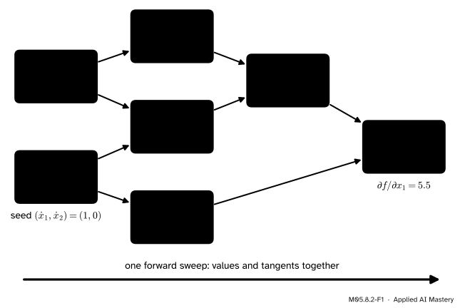
Forward mode on the running program with the seed \({(\dot x_1, \dot x_2) = (1, 0)}\): only \(x_1\) moves. Each node carries its value and its tangent, and the output’s tangent, 5.5, is \({\partial f / \partial x_1}\).
Moving only \(x_1\), at speed 1, makes the output’s speed exactly the partial derivative in \(x_1\). Moving only \(x_2\) gives the other partial derivative. Moving both in a direction \(\vect{r}\) gives the slope of \(f\) in that direction. Nothing is approximated: each tangent comes from an exact local derivative. This is forward-mode automatic differentiation.
Build it up
Step 1. Choose a direction: the seed. Pick a vector \(\vect{r}\) in input space and set the input tangents to it: \({\dot x_1 = r_1}\), \({\dot x_2 = r_2}\). This choice is the seed.
Step 2. Each operation has a tangent rule. If \({v = \varphi(u)}\) for one parent \(u\), then \({\dot v = \varphi'(u)\,\dot u}\): the chain rule of M04.3.4, read as “the speed of \(v\) is the local slope times the speed of \(u\)”. With two parents, the speeds add (the multivariable chain rule of M05.4):
\({v = u + w}\): \({\dot v = \dot u + \dot w}\); and \({v = u - w}\): \({\dot v = \dot u - \dot w}\).
\({v = u\,w}\): \({\dot v = \dot u\,w + u\,\dot w}\), the product rule.
\({v = u / w}\): \({\dot v = (\dot u\,w - u\,\dot w)/w^2}\), the quotient rule.
\({v = \ln u}\): \({\dot v = \dot u / u}\); \({v = e^u}\): \({\dot v = e^u\,\dot u}\).
Step 3. Sweep forward once. Walk down the trace in order, computing each value and then its tangent. The tangent rule only needs the values and tangents of the parents, which are already known. At the end, \(\dot y\) is the rate of change of the output along \(\vect{r}\).
Step 4. Let the numbers do the bookkeeping. Instead of writing a tangent rule beside every line, invent a new kind of number that carries a value and a tangent together and obeys the rules by itself. The trick is to see a tangent as the size of a tiny nudge.
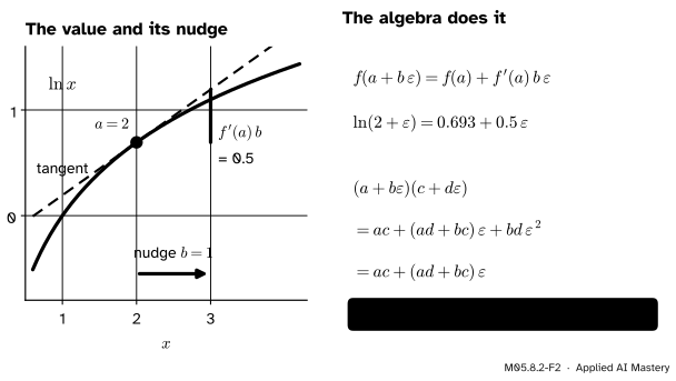
M05.8.2-F2
A dual number \({a + b\,\varepsilon}\) is a value \(a\) with a nudge of size \(b\) attached. A function moves the value to \(f(a)\) and the nudge to \({f'(a)\,b}\), as along the tangent line. Multiplying two dual numbers, the rule \({\varepsilon^2 = 0}\) throws away exactly the term the product rule leaves out.
The formal statement
NoteForward mode computes a Jacobian-vector product
Let \({f : \R^n \to \R^m}\) be computed by an evaluation trace of differentiable elementary operations, and seed the inputs with \({\dot{\vect{x}} = \vect{r}}\). Then each tangent is
Derivation. Move along the line \({\vect{x} + t\,\vect{r}}\) and treat every \(v_i\) as a function of the single number \(t\). The inputs move as \({x_j + t\,r_j}\), so their speeds at \({t = 0}\) are \(r_j\): the seed. Now suppose the speeds of all parents of \(v_i\) are known, and \({v_i = \varphi_i(u, w)}\) with parents \(u\) and \(w\). By the chain rule for a function of two moving inputs (M05.4.2),
\[
\begin{aligned}
\dot v_i &= \frac{d}{dt}\,\varphi_i(u(t), w(t)) \\
&= \pd{\varphi_i}{u}\,\dot u + \pd{\varphi_i}{w}\,\dot w .
\end{aligned}
\]
That is exactly the tangent rule of step 2. Every parent comes earlier in the trace, so going down the trace in order, every \(\dot v_i\) is the true speed of \(v_i\). The outputs are \({\vect{y}(t) = f(\vect{x} + t\,\vect{r})}\), and the derivative of \(f\) along a line is the Jacobian applied to the direction (M05.4.3): \({\dot{\vect{y}} = \mat{J}_f(\vect{x})\,\vect{r}}\).
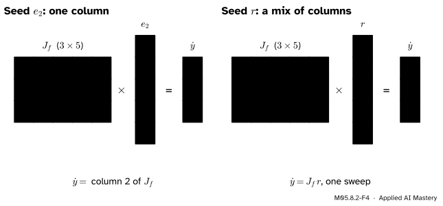
Consequences. With \({m = 1}\), \({\dot y = \nabla f(\vect{x})\T \vect{r}}\), the slope of \(f\) along \(\vect{r}\). With the seed \({\vect{r} = \vect{e}_j}\) the sweep returns column \(j\) of the Jacobian. So a full Jacobian, or a full gradient, takes \(n\) sweeps, one per input.
M05.8.2-F4
One forward sweep multiplies the Jacobian by the seed without ever forming the Jacobian. A basis seed picks out one column; any other seed mixes the columns.
NoteDual numbers
A dual number is \({a + b\,\varepsilon}\) with \(a\), \(b\) real and a new symbol \(\varepsilon\) that obeys \({\varepsilon^2 = 0}\) (and is not itself 0). For a differentiable \(f\) define
The definition is the linear approximation \({f(a + h) \approx f(a) + f'(a)\,h}\) (M04.2.2) with the nudge \({h = b\,\varepsilon}\). The Taylor terms in \(h^2\), \(h^3\), … all contain \(\varepsilon^2\), so they are 0, and the approximation becomes exact. Arithmetic follows from \({\varepsilon^2 = 0}\):
\[
\begin{aligned}
&(a + b\varepsilon)(c + d\varepsilon) \\
&\quad= ac + (ad + bc)\,\varepsilon + bd\,\varepsilon^2 \\
&\quad= ac + (ad + bc)\,\varepsilon .
\end{aligned}
\]
The \(\varepsilon\) part is the product rule. For division, multiply top and bottom by \({c - d\varepsilon}\), which makes the bottom \({c^2 - d^2\varepsilon^2 = c^2}\) (for \({c \neq 0}\)):
The \(\varepsilon\) part is the chain rule. So if every elementary operation is taught to act on dual numbers, any program built from them carries the tangent along by itself: put \({x_j + r_j\,\varepsilon}\) in, and read \(\mat{J}_f\vect{r}\) off the \(\varepsilon\) parts of the output.
Go deeper: dual numbers beside complex numbers
A complex number \({a + bi}\) is stored as the pair \({(a, b)}\) with \({i^2 = -1}\); a dual number is stored the same way with \({\varepsilon^2 = 0}\). The dual numbers can be written as the matrices \({\begin{pmatrix} a & b \\ 0 & a \end{pmatrix}}\): the matrix with \({a = 0}\), \({b = 1}\) squares to the zero matrix, and products of such matrices follow the dual rules. They were introduced by Clifford in 1873, long before automatic differentiation.
Worked example
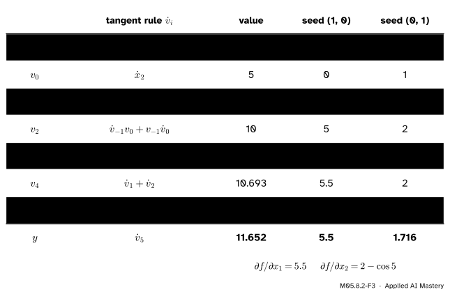
The running program at \({(2, 5)}\), seed \({(1, 0)}\). The values are those of M05.8.1. Go down the trace with the tangent rules:
\({\dot v_{-1} = 1}\) and \({\dot v_0 = 0}\), the seed.
\({\dot v_1 = \dot v_{-1} / v_{-1} = 1/2}\).
\({\dot v_2 = \dot v_{-1}\,v_0 + v_{-1}\,\dot v_0}\), which is \({1 \cdot 5 + 2 \cdot 0 = 5}\).
So \({\partial f/\partial x_1 = 5.5}\), which agrees with the hand derivative \({1/x_1 + x_2}\).
The same values, seed \({(0, 1)}\). Now \({\dot v_{-1} = 0}\) and \({\dot v_0 = 1}\), so \({\dot v_1 = 0}\), \({\dot v_2 = 0 \cdot 5 + 2 \cdot 1 = 2}\), \({\dot v_3 = \cos 5 \approx 0.284}\), \({\dot v_4 = 2}\) and \({\dot v_5 = 2 - \cos 5 \approx 1.716}\): the hand derivative \({x_1 - \cos x_2}\).
M05.8.2-F3
The tangent trace for two seeds. The values are computed once per sweep; the gradient \({(5.5,\ 1.716)}\) needs both sweeps, one per input.
Two inputs, two sweeps. A forward sweep costs a small multiple of one run of the program (each line does a little extra arithmetic), so the gradient in \(n\) inputs costs \(n\) sweeps, that small multiple of \(n\) runs. That is the same order as the \(2n\) runs of central differences. It is exact, but it still grows with \(n\).
Code
From scratch: a Dual class whose arithmetic follows the rules above. Python calls __add__, __mul__ and the rest whenever a Dual meets + or *, which is operator overloading: the program itself does not change.
import mathclass Dual:"""A dual number value + tangent * eps, with eps**2 = 0."""def__init__(self, value, tangent=0.0):self.value, self.tangent = value, tangent@staticmethoddef lift(x):return x ifisinstance(x, Dual) else Dual(x, 0.0) # a constant does not movedef__add__(self, other): o = Dual.lift(other)return Dual(self.value + o.value, self.tangent + o.tangent)__radd__=__add__def__neg__(self):return Dual(-self.value, -self.tangent)def__sub__(self, other):returnself+ (-Dual.lift(other))def__rsub__(self, other):return Dual.lift(other) -selfdef__mul__(self, other): o = Dual.lift(other)return Dual(self.value * o.value, self.tangent * o.value +self.value * o.tangent)__rmul__=__mul__def__truediv__(self, other): o = Dual.lift(other)return Dual(self.value / o.value, (self.tangent * o.value -self.value * o.tangent) / o.value **2)def__rtruediv__(self, other):return Dual.lift(other) /selfdef exp(x): x = Dual.lift(x)return Dual(math.exp(x.value), math.exp(x.value) * x.tangent)def ln(x): x = Dual.lift(x)return Dual(math.log(x.value), x.tangent / x.value)def sin(x): x = Dual.lift(x)return Dual(math.sin(x.value), math.cos(x.value) * x.tangent)def cos(x): x = Dual.lift(x)return Dual(math.cos(x.value), -math.sin(x.value) * x.tangent)def tanh(x): x = Dual.lift(x) th = math.tanh(x.value)return Dual(th, (1- th * th) * x.tangent)def f(x1, x2): # the running program, written as plain codereturn ln(x1) + x1 * x2 - sin(x2)for seed in ((1.0, 0.0), (0.0, 1.0), (0.6, 0.8)): y = f(Dual(2.0, seed[0]), Dual(5.0, seed[1]))print(f"seed {seed}: value {y.value:.3f}, tangent {y.tangent:.3f}")
seed (1.0, 0.0): value 11.652, tangent 5.500
seed (0.0, 1.0): value 11.652, tangent 1.716
seed (0.6, 0.8): value 11.652, tangent 4.673
The seed \({(0.6, 0.8)}\) is the unit direction \({(3, 4)/5}\), and its single sweep gives the slope of \(f\) in that direction, about 4.673, which is \({0.6 \times 5.5 + 0.8 \times 1.716}\).
Now a check against central differences on functions that use every operation, at random points, and the running chain of M04.3.4, whose slope \({dE/dw \approx -0.212}\) came from multiplying local slopes by hand:
import numpy as npdef g(x1, x2):return exp(x1 / x2) * tanh(x1 -2* x2) + cos(x1 * x2)rng = np.random.default_rng(0)worst =0.0for _ inrange(100): a, b = rng.uniform(0.5, 2.0, size=2) h =1e-6for seed, fd in (((1.0, 0.0), (g(a + h, b).value - g(a - h, b).value) / (2* h)), ((0.0, 1.0), (g(a, b + h).value - g(a, b - h).value) / (2* h))): worst =max(worst, abs(g(Dual(a, seed[0]), Dual(b, seed[1])).tangent - fd))print("largest gap to central differences over 200 slopes:", f"{worst:.1e}")def sigmoid(z):return1/ (1+ exp(-z))w = Dual(0.5, 1.0) # the weight moves at speed 1; x = 2 and y = 1 are constantsr = sigmoid(w *2.0) -1.0E = r * rprint(f"running chain: E = {E.value:.3f}, dE/dw = {E.tangent:.3f}")
largest gap to central differences over 200 slopes: 7.9e-09
running chain: E = 0.072, dE/dw = -0.212
Last, a map with two outputs, the warp \({(x, y) \mapsto (x + 0.3\sin y,\; y + 0.3\sin x)}\) of M05.4, at \({(1, 2)}\). Each sweep returns one column of its Jacobian, and two sweeps are compared with scipy.differentiate.jacobian, which estimates the whole matrix by finite differences:
from scipy.differentiate import jacobiandef warp(x, y):return [x +0.3* sin(y), y +0.3* sin(x)]columns = []for seed in ((1.0, 0.0), (0.0, 1.0)): out = warp(Dual(1.0, seed[0]), Dual(2.0, seed[1])) columns.append([o.tangent for o in out])J_forward = np.array(columns).Tdef warp_np(p): # the same map on NumPy arrays, for SciPyreturn np.array([p[0] +0.3* np.sin(p[1]), p[1] +0.3* np.sin(p[0])])J_scipy = jacobian(warp_np, np.array([1.0, 2.0])).dfprint(np.round(J_forward, 4))print("agrees with SciPy:", np.allclose(J_forward, J_scipy, atol=1e-8))
The Jacobian \({\begin{pmatrix} 1 & 0.3\cos y \\ 0.3\cos x & 1 \end{pmatrix}}\) comes out column by column, \({(1,\ 0.1621)}\) from the first sweep and \({(-0.1248,\ 1)}\) from the second. In libraries this is jax.jvp, which takes a function, a point and a seed and returns the value and \(\mat{J}_f\vect{r}\) together.
Explore
The module’s interactive, the graph stepper, lives in lesson M05.8.3. Choose its forward mode, pick the seed \({(1, 0)}\) and step through the nodes: each one fills in its value and its tangent. Then switch to the seed \({(0, 1)}\) and run a second sweep; the read-out counts how many sweeps the full gradient has cost.
Pitfalls
M05.8.2-F5
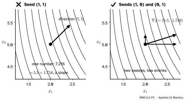
Wrong beside right. Seeding both inputs with 1 returns one number, the rate of change along \({(1, 1)}\). The gradient needs one sweep per input; its arrow (drawn at 0.13 of its length) is built from the two answers.
“Seed every input with 1 and you get the whole gradient in one sweep.”
The output tangent is \({\nabla f\T\vect{r}}\), one number. With \({\vect{r} = (1, 1)}\) it is \({5.5 + 1.716 = 7.216}\), the sum of the partial derivatives, and the separate entries cannot be recovered from it. Forward mode gets one number per sweep per output; a gradient of length \(n\) needs \(n\) sweeps.
“\(\varepsilon\) is a very small number, like the \(h\) of a finite difference.”
It is not a number on the real line at all. It is a symbol with the rule \({\varepsilon^2 = 0}\), and that rule removes the higher Taylor terms exactly. There is no step to choose and no subtraction of nearly equal values, so there is no rounding trouble of the kind M04.2.4 showed.
“Every number in the program needs a tangent of 1.”
A constant, such as the 4 in \({4\,l(1 - l)}\) or the fixed input \(x\) of the running chain, does not move when the inputs move, so its tangent is 0. Giving it a tangent changes the question: the answer becomes a derivative in a direction that also moves that constant.
Check yourself
Recall
1. What does the tangent \(\dot v_i\) of a variable measure?
Show answer
The rate at which \(v_i\) changes when the inputs move along the seed direction \(\vect{r}\): \({\dot v_i = \tfrac{d}{dt}\,v_i(\vect{x} + t\vect{r})}\) at \({t = 0}\).
2. What is the tangent rule for \({v = u\,w}\)?
Show answer
\({\dot v = \dot u\,w + u\,\dot w}\), the product rule.
3. What does one forward sweep with seed \(\vect{r}\) compute?
Show answer
The values of the program and the Jacobian-vector product \({\mat{J}_f(\vect{x})\,\vect{r}}\); for a scalar output, the slope \({\nabla f\T\vect{r}}\) along \(\vect{r}\).
4. Why is \({f(a + b\varepsilon) = f(a) + f'(a)\,b\,\varepsilon}\) exact rather than approximate?
Show answer
Every Taylor term beyond the linear one contains \(\varepsilon^2\) or a higher power, and \({\varepsilon^2 = 0}\).
5. How many forward sweeps does the gradient of a function of \(n\) inputs need?
Show answer
\(n\), one per basis seed \(\vect{e}_j\), each giving one partial derivative.
Exercises
1.★ Compute \({(3 + 2\varepsilon)(1 - \varepsilon)}\) and \({(3 + 2\varepsilon)/(1 - \varepsilon)}\). Check the second with the quotient rule for \({u/w}\) with \({u = 3 + 2t}\) and \({w = 1 - t}\) at \({t = 0}\).
Show solution
Product, with \({a = 3}\), \({b = 2}\), \({c = 1}\), \({d = -1}\): the value part is \({ac = 3}\) and the \(\varepsilon\) part is
\[
ad + bc = 3 \cdot (-1) + 2 \cdot 1 = -1,
\]
so the product is \({3 - \varepsilon}\). Quotient: the value part is \({a/c = 3}\) and the \(\varepsilon\) part is
so the quotient is \({3 + 5\varepsilon}\). At \({t = 0}\) the quotient rule \({(u'w - uw')/w^2}\) gives \({(2 + 3)/1 = 5}\), the same \(\varepsilon\) part.
2.★★ Run forward mode by hand on \({g(x_1, x_2) = x_1 \tanh x_2}\) at \({(2, 0.5)}\) with the seed \({(0, 1)}\). Give every value and tangent to three decimals.
Show solution
\({v_{-1} = 2}\), \({\dot v_{-1} = 0}\); \({v_0 = 0.5}\), \({\dot v_0 = 1}\). \({v_1 = \tanh v_0 \approx 0.462}\), and its tangent is \({1 - \tanh^2 0.5 \approx 0.786}\). \({v_2 = v_{-1} v_1 \approx 0.924}\), and \({\dot v_2 = \dot v_{-1} v_1 + v_{-1} \dot v_1}\), which is \({0 + 2 \times 0.786 \approx 1.573}\). So \({\partial g/\partial x_2 \approx 1.573}\), the value of \({x_1(1 - \tanh^2 x_2)}\).
3.★★★ Show that each tangent is linear in the seed: the sweep with seed \({a\vect{r} + b\vect{s}}\) gives \(a\) times the tangents for \(\vect{r}\) plus \(b\) times those for \(\vect{s}\). Use it to find the slope of the running program along \({(3, 4)/5}\) from the two sweeps of the worked example.
Show solution
Induction down the trace. The input tangents are the seed, so the claim holds for them. Each tangent rule has the form \({\dot v_i = \sum_u \pd{\varphi_i}{u}\,\dot u}\), where the local derivatives depend only on the values, which are the same in every sweep. A fixed combination of the parents’ tangents is linear in them, and they are linear in the seed by the induction hypothesis, so \(\dot v_i\) is too. For \({(3, 4)/5 = 0.6\,\vect{e}_1 + 0.8\,\vect{e}_2}\) the slope is \({0.6 \times 5.5 + 0.8 \times 1.716 \approx 4.673}\), which the code finds with a single sweep.
Summary card
Forward mode carries a tangent beside every value.
M05.8.2-F1
Values and tangents in one forward sweep.
Tangent rule: \({\dot v = \varphi'(u)\,\dot u}\), summed over the parents.
One sweep with seed \(\vect{r}\) gives \({\mat{J}_f\vect{r}}\); the gradient needs \(n\) sweeps.
Sources. Each was opened and checked against this lesson on 15 November 2026.
A. G. Baydin, B. A. Pearlmutter, A. A. Radul and J. M. Siskind, Automatic Differentiation in Machine Learning: a Survey, JMLR 18(153), 2018. Section 3.1 and Table 2: the forward tangent trace of the running program at \({(2, 5)}\) with \({\dot x_1 = 1}\), ending in \({\dot y = 5.5}\); seeding with \({\dot{\vect{x}} = \vect{r}}\) gives the Jacobian-vector product (their equation 4), and the gradient takes \(n\) evaluations. Section 3.1.1: dual numbers \({v + \dot v\varepsilon}\) with \({\varepsilon^2 = 0}\), the rule \({f(v + \dot v\varepsilon) = f(v) + f'(v)\dot v\varepsilon}\) (their equation 5), the chain rule through compositions, and Clifford (1873). Their tangent is our \(\dot v_i\).
P. Bright, A. Edelman and S. G. Johnson, Matrix Calculus (for Machine Learning and Beyond), section 8.1: forward mode by a new number type carrying a value and a derivative, and in 8.1.3 the dual number \({a + b\varepsilon}\) with the sum, product and quotient rules derived from \({\varepsilon^2 = 0}\).