Run the program forward and record a tape, then sweep backward with adjoints, the derivative of the output with respect to each intermediate value. One backward sweep gives every partial derivative at once; adjoints add where a value is used twice.
M05.8.3L2 Intermediate25 minIn review (what this means)
The maths and code on this page are checked by automated tests on every change, but an independent reader has not signed it off yet. Spot a mistake or a confusing step? Tell us.
Define the adjoint of an intermediate variable as the derivative of the output with respect to it, and state how it is passed back to the variable’s parents.
Derive the adjoint recurrence from the path-sum form of the chain rule, including the sum where a value is used twice.
Run a reverse-mode sweep by hand on a small trace and read off the whole gradient.
Implement reverse mode with a scalar Var class, a topological sort and a backward method, and check it with scipy.optimize.check_grad.
The question
Forward mode answers “if the inputs move this way, how fast does every value move?”, and needs one sweep per input. A loss has one output and maybe a billion inputs. Ask the question the other way round: “how much does the output care about each value?” Can that question be answered for every value in the program at once?
From the last lesson
1. What does one forward-mode sweep with seed \(\vect{r}\) compute?
Show answer
The values of the program and the Jacobian-vector product \({\mat{J}_f(\vect{x})\,\vect{r}}\); for a scalar output, the slope along \(\vect{r}\).
2. What is the tangent rule for \({v = u\,w}\)?
Show answer
\({\dot v = \dot u\,w + u\,\dot w}\).
Intuition
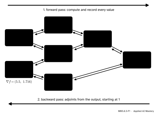
Give every value \(v\) in the program a second number, its adjoint\(\delta_v\): how much the output \(y\) would change per unit change of \(v\), everything downstream of \(v\) reacting. The output cares about itself exactly one-for-one, so \({\delta_y = 1}\). A value one step before the output matters through that last step only, so its adjoint is the output’s adjoint times the local derivative of the last step. And so on, backwards through the graph.
M05.8.3-F1
The two passes of reverse mode on the running program. The forward pass computes and records the values; the backward pass starts with \({\delta = 1}\) at the output and sends adjoints back along every edge. The adjoints of the inputs are the gradient.
The striking thing is the bottom-left corner. One backward sweep fills in the adjoint of every node, and the inputs are nodes, so both partial derivatives arrive together. With a billion inputs, it would still be one backward sweep. This is reverse-mode automatic differentiation, and backpropagation in a neural network is exactly this (M05.9).
Build it up
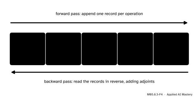
Step 1. Record the forward pass. Run the program once and keep, for every node, its value, its parents and the local derivative to each parent, \({\partial v / \partial u}\). For \({v_2 = v_{-1} v_0}\) at \({(2, 5)}\) the local derivatives are \({v_0 = 5}\) and \({v_{-1} = 2}\): they need the values, which is why they are recorded on the way forward. This record is the tape.
Step 2. Seed the output.\({\delta_y = 1}\), since \({\partial y/\partial y = 1}\). Every other adjoint starts at 0.
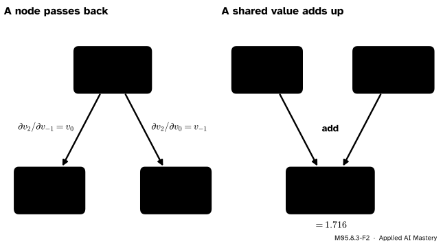
Step 3. A node passes its adjoint back. When a node \(v\) is reached, it sends \({\delta_v \cdot \partial v/\partial u}\) to each parent \(u\): its own importance, times how strongly it depends on that parent.
Step 4. A value used twice collects twice. The input \(x_2\) feeds both the product \(v_2\) and the sine \(v_3\), so a change in \(x_2\) reaches the output along two routes, and the two effects add.
M05.8.3-F2
Left: a product passes its adjoint to each factor, times the other factor. Right: \(x_2\) is used by two nodes, so its adjoint is the sum of what they send: \({2 + (-1)\cos 5 \approx 1.716}\).
Step 5. Go in reverse order. A node must have received everything from its children before it passes anything on. Walking the tape from its last line to its first guarantees this, because every child of a node comes later in the trace.
The formal statement
NoteThe adjoint recurrence
For a scalar output \(y\) of an evaluation trace, the adjoint of a variable \(v_i\) is \({\delta_{v_i} = \partial y / \partial v_i}\), the derivative of \(y\) when \(v_i\) is changed and every variable computed from it is recomputed. Then \({\delta_y = 1}\), and for every other variable
\[
\cgrad{\delta_{v_i}} = \sum_{j \,:\, v_i \text{ is a parent of } v_j} \cgrad{\delta_{v_j}}\, \pd{v_j}{v_i} .
\]
Computing the adjoints in reverse order of the trace gives all of them in one backward sweep; those of the inputs are the gradient \({\nabla f(\vect{x})}\).
Derivation. The chain rule on a graph (the tree diagrams of M05.4.2, and the path sums in the entries of a Jacobian product in M05.4.3) says that a derivative of one variable with respect to an earlier one is a sum over paths: for every path from \(v_i\) to \(y\), multiply the local derivatives along its edges, and add the products over all paths,
Every path from \(v_i\) starts with one edge, to one of its children \(v_j\), and then continues as a path from \(v_j\) to \(y\). Group the paths by that first edge. The factor \({\partial v_j/\partial v_i}\) is common to the group, and what remains is the sum over all paths from \(v_j\) to \(y\), which is \({\partial y/\partial v_j = \delta_{v_j}}\):
The children of \(v_i\) all come after it in the trace. So when the trace is walked from the end, each \(\delta_{v_j}\) on the right is finished before \(\delta_{v_i}\) is needed. In practice the sum is built up the other way round, as in step 3: each node, when reached, adds its contribution \({\delta_{v_j}\,\partial v_j/\partial v_i}\) to each parent’s running adjoint, an update written \({\delta_{v_i} \mathrel{+}= \dots}\) in code. Both give the same sums.
The cost. The backward sweep visits every edge once, with one multiplication and one addition, and the local derivatives were found on the way forward. So the whole gradient costs a small constant times one run of \(f\), whatever the number of inputs. The price is memory: the tape holds every value until the backward sweep is over. Lesson M05.8.4 weighs the two.
Go deeper: many outputs: vector-Jacobian products
If \({f : \R^n \to \R^m}\), seed the output adjoints with a vector \(\vect{u}\) instead of 1. The recurrence is linear in the seed, so by the path sums each adjoint becomes \({\delta_{v_i} = \sum_k u_k\,\partial y_k/\partial v_i}\), and the input adjoints are \({\sum_k u_k \nabla y_k = \mat{J}_f\T\vect{u}}\), a vector-Jacobian product. The seed \({\vect{u} = \vect{e}_k}\) gives row \(k\) of the Jacobian, so the full Jacobian takes \(m\) backward sweeps. Exercise 3 asks for the details.
Worked example
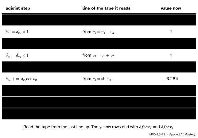
The running program at \({(2, 5)}\). The forward pass gives the values of M05.8.1 and the local derivatives: \({\partial v_1/\partial v_{-1} = 1/2}\), \({\partial v_2/\partial v_{-1} = v_0 = 5}\), \({\partial v_2/\partial v_0 = v_{-1} = 2}\), \({\partial v_3/\partial v_0 = \cos 5 \approx 0.284}\), 1 for both inputs of \(v_4\), and \({+1}\) and \({-1}\) for the inputs of \({v_5 = v_4 - v_3}\). Now walk back:
M05.8.3-F3
The backward sweep, line by line. Each input’s adjoint is built up from two contributions, one per use of the input.
From \({v_2 = v_{-1} v_0}\): \(\delta_{v_{-1}}\) receives \({1 \times 5 = 5}\), and \(\delta_{v_0}\) receives \({1 \times 2 = 2}\), so \({\delta_{v_0} = 2 - \cos 5 \approx 1.716}\).
From \({v_1 = \ln v_{-1}}\): \(\delta_{v_{-1}}\) receives \({1 \times 1/2}\), so \({\delta_{v_{-1}} = 5.5}\).
One backward sweep, and the gradient \({(5.5,\ 1.716)}\) is complete; forward mode needed two sweeps for the same two numbers.
The running chain of M04.3.4. With \({r = p - y}\) and \({E = r^2}\): \({\delta_E = 1}\), \({\delta_r = 2r \approx -0.538}\), \({\delta_p = \delta_r \approx -0.538}\), \({\delta_z = \delta_p\,p(1 - p)}\), which is \({-0.538 \times 0.197 \approx -0.106}\), and \({\delta_w = \delta_z \cdot x \approx -0.212}\). These are the running products of local slopes that lesson M04.3.4 called the backward pass. On a chain, reverse mode is that walk; on a graph, the only new rule is to add at a fork.
Code
From scratch: a scalar class Var that records, for every result, its parents and the local derivatives. backward sorts the graph topologically (parents before children), then plays it in reverse, adding adjoints.
M05.8.3-F4
The tape of the running program. Each record holds what the backward pass will need: the parents and the local slopes, evaluated at the forward values. The Var class keeps the same records inside its objects.
import mathclass Var:"""A scalar that remembers its parents and the local derivative to each one."""def__init__(self, value, parents=()):self.value, self.parents, self.adjoint = value, parents, 0.0@staticmethoddef lift(x):return x ifisinstance(x, Var) else Var(x) # a constant has no parentsdef__add__(self, other): o = Var.lift(other)return Var(self.value + o.value, ((self, 1.0), (o, 1.0)))__radd__=__add__def__neg__(self):return Var(-self.value, ((self, -1.0),))def__sub__(self, other):returnself+ (-Var.lift(other))def__rsub__(self, other):return Var.lift(other) -selfdef__mul__(self, other): o = Var.lift(other)return Var(self.value * o.value, ((self, o.value), (o, self.value)))__rmul__=__mul__def__truediv__(self, other): o = Var.lift(other)return Var(self.value / o.value, ((self, 1/ o.value), (o, -self.value / o.value **2)))def__rtruediv__(self, other):return Var.lift(other) /selfdef backward(self): order, seen, stack = [], set(), [(self, False)]while stack: # depth-first topological sort v, finished = stack.pop()if finished: order.append(v) # listed after all its parentselifid(v) notin seen: seen.add(id(v)) stack.append((v, True)) stack += [(p, False) for p, _ in v.parents ifid(p) notin seen]for v in order: v.adjoint =0.0self.adjoint =1.0for v inreversed(order): # the tape, played backwardsfor parent, local in v.parents: parent.adjoint += v.adjoint * local # add, never overwritedef exp(x):return Var(math.exp(x.value), ((x, math.exp(x.value)),))def ln(x):return Var(math.log(x.value), ((x, 1/ x.value),))def sin(x):return Var(math.sin(x.value), ((x, math.cos(x.value)),))def cos(x):return Var(math.cos(x.value), ((x, -math.sin(x.value)),))def tanh(x): th = math.tanh(x.value)return Var(th, ((x, 1- th * th),))x1, x2 = Var(2.0), Var(5.0)y = ln(x1) + x1 * x2 - sin(x2)y.backward()print(f"y = {y.value:.3f}, gradient = ({x1.adjoint:.3f}, {x2.adjoint:.3f})")
y = 11.652, gradient = (5.500, 1.716)
The running chain, where x and y are plain numbers and only the weight is a Var:
Now a function of five inputs, built from every operation, checked with scipy.optimize.check_grad. It compares our gradient with a forward-difference estimate and returns the length of the difference, so a small number means agreement.
import numpy as npfrom scipy.optimize import check_graddef F(x): chain =sum(tanh(x[i] * x[i +1]) for i inrange(len(x) -1))return chain + ln(1+ x[0] * x[0]) + exp(x[-1] /3) * cos(x[2])def value(x):return F([Var(v) for v in x]).valuedef gradient(x): xs = [Var(v) for v in x] F(xs).backward()return np.array([v.adjoint for v in xs])x0 = np.array([0.3, -1.2, 0.8, 2.0, -0.5])print("gradient by one backward sweep:", np.round(gradient(x0), 4))print("check_grad (length of the gap):", f"{check_grad(value, gradient, x0):.1e}")
gradient by one backward sweep: [-0.5065  0.6211 -0.8414 -0.0896  1.0365]
check_grad (length of the gap): 2.9e-08
The gap is of the size a forward difference with step about \({1.5 \times 10^{-8}}\) makes; the reverse-mode gradient is the exact one, up to rounding. In libraries the same sweep is loss.backward() in PyTorch or jax.grad(f) in JAX; DL01.6 builds a fuller engine of this kind.
Explore
M05.8-X1
Graph stepper
Set \(x_1\) and \(x_2\) with the sliders, choose forward or reverse mode, and step through the graph one node at a time. In forward mode, pick a seed and watch values and tangents fill in together; in reverse mode, a forward pass fills in the values, then a backward pass fills in the adjoints.
Three things to try. In forward mode with the seed \({(1, 0)}\) at \({(2, 5)}\), the output’s tangent is 5.5; then run the seed \({(0, 1)}\) and see the sweep count reach 2. In reverse mode, notice that \(x_2\)’s adjoint changes twice during the backward pass, once from \(v_3\) and once from \(v_2\). And watch the read-out compare the sweeps each method needs: forward mode 2, reverse mode 1, central differences 4 runs of \(f\).
Pitfalls
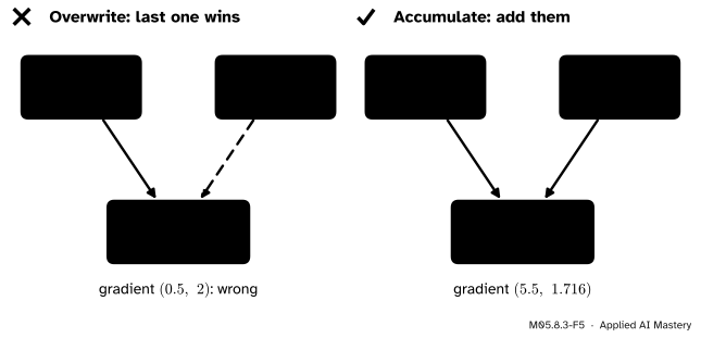
M05.8.3-F5
Wrong beside right. If each contribution replaces the adjoint instead of adding to it, \(x_2\) keeps only the last one, 2, and \(x_1\) only \({1/2}\).
“Set the parent’s adjoint to what the child sends.”
A value used twice must collect both contributions. Overwriting gives \({(0.5,\ 2)}\) for the running program instead of \({(5.5,\ 1.716)}\), and the error is silent: the numbers look reasonable. In a network, a shared weight (a convolution filter, a tied embedding) is exactly such a value. M05.9.3 catches this bug with a gradient check.
“The backward pass can run without the forward pass.”
The local derivatives depend on the values: \({\partial v_2/\partial v_{-1} = v_0}\) and \({\partial v_3/\partial v_0 = \cos v_0}\). Without a forward pass there is nothing to multiply by. That is why the tape is recorded, and why reverse mode needs memory for every value of the trace.
“Reverse mode gives the whole Jacobian in one sweep.”
It gives the gradient of one output in one sweep: one row of the Jacobian. A function with \(m\) outputs needs \(m\) backward sweeps for its full Jacobian, just as forward mode needs \(n\) forward sweeps. A loss has \({m = 1}\), which is why reverse mode wins in training.
Check yourself
Recall
1. What is the adjoint \(\delta_v\) of a variable?
Show answer
The derivative of the output with respect to \(v\), \({\partial y/\partial v}\), with everything computed from \(v\) allowed to react.
2. What does a node \(v_j\) send back to its parent \(v_i\)?
Show answer
\({\delta_{v_j}\,\partial v_j/\partial v_i}\): its adjoint times its local derivative to that parent.
3. Why are the adjoints of a value used twice added?
Show answer
Every path from the value to the output starts with one of its uses, and the chain rule on a graph sums over all paths; grouping the paths by their first edge gives one term per use.
4. Why must the forward pass come first and be recorded?
Show answer
The local derivatives depend on the values (for example \({\partial(uw)/\partial u = w}\)), and the backward sweep needs the order of the trace.
5. What gradient does one backward sweep give for the running program at \({(2, 5)}\)?
Show answer
\({(5.5,\ 2 - \cos 5) \approx (5.5,\ 1.716)}\), both entries in one sweep.
Exercises
1.★ Write the trace of \({g(x_1, x_2) = x_1 x_2 + x_1}\) and run reverse mode by hand at \({(3, 4)}\). Check against the partial derivatives.
Show solution
\({v_{-1} = 3}\), \({v_0 = 4}\), \({v_1 = v_{-1} v_0 = 12}\), \({v_2 = v_1 + v_{-1} = 15}\). Backward: \({\delta_{v_2} = 1}\); from \(v_2\), \({\delta_{v_1} = 1}\) and \(\delta_{v_{-1}}\) receives 1; from \(v_1\), \(\delta_{v_{-1}}\) receives \({1 \times v_0 = 4}\), so \({\delta_{v_{-1}} = 5}\), and \({\delta_{v_0} = 1 \times v_{-1} = 3}\). The partial derivatives are \({x_2 + 1 = 5}\) and \({x_1 = 3}\).
2.★★ The log loss of one positive example is \({E = -\ln \sigma(z)}\) with \({z = w x + b}\). Run reverse mode at \({w = 0.5}\), \({b = 0}\), \({x = 2}\), and show that \({\delta_z = \sigma(z) - 1}\).
Show solution
Forward: \({z = 1}\), \({p = \sigma(1) \approx 0.731}\), \({E = -\ln p \approx 0.313}\). Backward: \({\delta_E = 1}\), \({\delta_p = -1/p \approx -1.368}\), \({\delta_z = \delta_p\,p(1 - p)}\), which simplifies to \({-(1 - p) = p - 1 \approx -0.269}\), then \({\delta_w = \delta_z\,x \approx -0.538}\) and \({\delta_b = \delta_z \approx -0.269}\). The factor \(p(1 - p)\) cancels against \({1/p}\), the simplification M05.9.1 relies on.
3.★★★ For \({f : \R^n \to \R^m}\), seed the backward sweep with output adjoints \({\vect{u} \in \R^m}\). Show that the input adjoints are \({\mat{J}_f(\vect{x})\T\vect{u}}\), and conclude how many sweeps the full Jacobian needs.
Show solution
With several outputs, the backward recurrence for the working variables is unchanged, and each output \(y_k\) starts with \({\delta_{y_k} = u_k}\). Every quantity in the sweep is a sum of products with exactly one factor \(u_k\), so the result is linear in \(\vect{u}\): it is the sum over \(k\) of \(u_k\) times the sweep seeded with \(\vect{e}_k\). Seeded with \(\vect{e}_k\), the sweep is the single-output sweep of \(y_k\), which gives \({\nabla y_k}\). So the input adjoints are \({\sum_k u_k\,\nabla y_k}\). The rows of \(\mat{J}_f\) are \({\nabla y_k\T}\), so this sum is \({\mat{J}_f\T\vect{u}}\). With \({\vect{u} = \vect{e}_k}\) the sweep returns row \(k\), so the whole Jacobian takes \(m\) backward sweeps.
Summary card
Reverse mode: forward to record, backward to collect adjoints.
M05.8.3-F1
One backward sweep, the whole gradient.
Adjoint: \({\delta_v = \partial y/\partial v}\), with \({\delta_y = 1}\).
Recurrence: \({\delta_{v_i} = \sum_j \delta_{v_j}\,\partial v_j/\partial v_i}\) over the children.
Adjoints add where a value is used twice.
Cost: a small multiple of one run; memory: the whole tape.
Sources and next steps
Sources. Each was opened and checked against this lesson on 15 November 2026.
A. G. Baydin, B. A. Pearlmutter, A. A. Radul and J. M. Siskind, Automatic Differentiation in Machine Learning: a Survey, JMLR 18(153), 2018. Section 3.2 defines the adjoint \({\bar v_i = \partial y_j/\partial v_i}\) (we write \(\delta_{v_i}\), keeping the overbar for means), describes the two phases, and shows the contribution of \(v_0\) through \(v_2\) and \(v_3\) added in two incremental steps; Table 3 gives the reverse adjoint trace at \({(2, 5)}\), ending in 5.5 and 1.716; the section also notes the storage cost and the transposed Jacobian-vector product.
P. Bright, A. Edelman and S. G. Johnson, Matrix Calculus (for Machine Learning and Beyond): section 8.3.1 gives the reverse-mode rule \({\partial z/\partial a = \sum_i (\partial b_i/\partial a)(\partial z/\partial b_i)}\) over the nodes \(b_i\) that \(a\) influences; section 8.4 describes the tape that is played backwards.
M. P. Deisenroth, A. A. Faisal and C. S. Ong, Mathematics for Machine Learning, section 5.6.2: Example 5.14 works backwards from the output through a computation graph, and equation (5.145) sums over the children of a node.
SciPy, scipy.optimize.check_grad: returns the 2-norm of the difference between a gradient and a forward-difference estimate, with default step \({\sqrt{\text{machine epsilon}} \approx 1.49 \times 10^{-8}}\).