Any program built from elementary operations is a directed acyclic graph, and running it leaves an evaluation trace of intermediate values. Build the trace and the graph of ln x1 + x1 x2 - sin x2 by hand, and see why neither finite differences nor symbolic algebra suits training.
M05.8.1L2 Intermediate25 minIn review (what this means)
The maths and code on this page are checked by automated tests on every change, but an independent reader has not signed it off yet. Spot a mistake or a confusing step? Tell us.
Break a formula or a short program into an evaluation trace of elementary operations with intermediate variables v_i.
Draw the computational graph of a trace and evaluate it in a topological order.
Explain how loops and branches unroll into a trace for the inputs actually given.
Explain why finite differences (2n evaluations and rounding error) and symbolic differentiation (expression swell) do not suit training.
The question
A language model has billions of weights, and every training step needs the slope of the loss in each one of them. Nudging the weights one at a time would take billions of runs of the model per step. Yet a library returns all of those slopes for about the price of a couple of runs. What does it see in your code that makes this possible?
Intuition
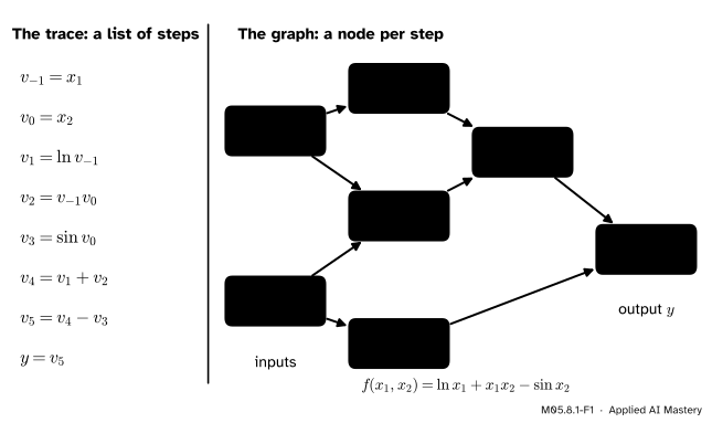
A computer never evaluates a formula in one go. It runs a sequence of tiny steps, each one an operation it knows well: add, multiply, take a logarithm, a sine, an exponential. Write each step on its own line and give its result a name, and you have the evaluation trace of the program. Draw each step as a node, with an arrow from every value to each step that uses it, and you have its computational graph.
M05.8.1-F1
The running program of this module, \({f(x_1, x_2) = \ln x_1 + x_1 x_2 - \sin x_2}\), as a trace (left) and as a graph (right). Each line of the trace is one node; each arrow says “this value is used here”.
The two pictures hold the same information. The trace is the order in which the computer did the work. The graph shows what depends on what. Both are made of pieces whose derivatives we already know, joined by the chain rule (M04.3.4, and its many-variable form in M05.4). That is the whole secret of automatic differentiation: differentiate each tiny step, and let the graph say how to combine the results. This lesson builds the graph; the next three run derivatives through it.
Build it up
Step 1. Name every intermediate result. Take \({f(x_1, x_2) = \ln x_1 + x_1 x_2 - \sin x_2}\), the worked example of section 3 of the survey by Baydin et al. Following their numbering, the inputs get the indices \({-1}\) and \({0}\), so that the working variables start at 1: \({v_{-1} = x_1}\) and \({v_0 = x_2}\). Then each operation gets the next index: \({v_1 = \ln v_{-1}}\), \({v_2 = v_{-1} v_0}\), \({v_3 = \sin v_0}\), \({v_4 = v_1 + v_2}\) and \({v_5 = v_4 - v_3}\). The output is \({y = v_5}\). This list is also called a Wengert list, after the man who used it in 1964 to compute derivatives automatically.
Step 2. Each line uses only earlier lines. That is what makes it a program that can run: when the computer reaches line \(v_4\), the values \(v_1\) and \(v_2\) already exist. In the graph, it means every arrow points from an earlier node to a later one, so no path ever leads back to where it started. A graph with that property is a directed acyclic graph, a DAG.
Step 3. A value used twice is one node with two arrows out. The input \(x_1\) feeds both the logarithm and the product. In the graph it is one node, \(v_{-1}\), with two outgoing arrows. This sharing will matter in lesson M05.8.3, where derivatives flowing back along both arrows must be added.
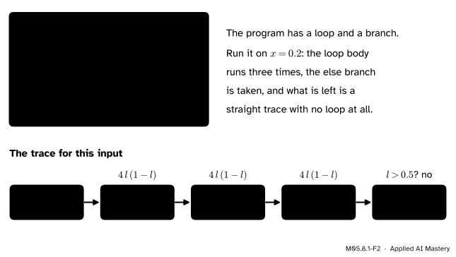
Step 4. Loops and branches disappear. A real program has for loops and if statements. But any single run, on particular inputs, executes particular lines in a particular order. Record them and the loop is unrolled, and only the branch actually taken appears.
M05.8.1-F2
A loop of three passes of the logistic map \({l \mapsto 4l(1 - l)}\), followed by a branch. For the input \({x = 0.2}\) the run leaves a straight chain: each pass becomes three elementary steps, and the branch not taken leaves no trace.
The trace depends on the input: for \({x = 0.3}\) the third pass gives about 0.9943, the test \({l > 0.5}\) passes, and the other branch is recorded. A derivative computed from a trace is the derivative of the function along that path. At an input where the test switches, the function can jump, and no method of differentiation can give a slope there.
The formal statement
NoteDefinition: evaluation trace and computational graph
Let \({f : \R^n \to \R^m}\) be computed by a program built from elementary operations. An evaluation trace of \(f\) at a point is a list of variables
the inputs \({v_{i-n} = x_i}\) for \({i = 1, \dots, n}\),
the working variables \({v_i = \varphi_i(\text{parents of } v_i)}\) for \({i = 1, \dots, \ell}\), where each \(\varphi_i\) is an elementary operation and every parent of \(v_i\) has a smaller index,
and the outputs, which are the last \(m\) working variables.
The computational graph has one node per variable and an edge from \(v_j\) to \(v_i\) whenever \(v_j\) is a parent of \(v_i\). It is a directed acyclic graph.
The elementary operations are those whose derivatives are known exactly: addition, subtraction, multiplication, division, and functions such as \(\exp\), \(\ln\), \(\sin\), \(\cos\), \(\tanh\) and the sigmoid \(\sigma\) (whose slope \({\sigma(1 - \sigma)}\) is M04.3.3).
Why the graph has no cycle. An edge from \(v_j\) to \(v_i\) means \({j < i}\). Along any path the index rises at every step, so a path can never come back to the node it started from.
Evaluating a graph. A topological order is a list of all the nodes in which each node comes after all of its parents. The trace is one such order. Evaluating the nodes in any topological order computes the same values, because each node then sees exactly the values of its parents, and those do not depend on the order. When a graph arrives as a set of nodes in no particular order, a topological order can always be found.
Go deeper: every directed acyclic graph has a topological order
First, a finite DAG has a node with no parents. Suppose instead that every node had a parent. Start anywhere and keep stepping to a parent. You never get stuck, and there are only finitely many nodes, so some node is visited twice. The steps between the two visits form a cycle, which a DAG does not have.
Now build the order: take a node with no parents, put it next in the list, and delete it with its edges. What remains is still a finite DAG (deleting cannot create a cycle), so it again has a node with no parents. Repeat until no nodes remain. Each node enters the list only after all its parents have been deleted, which means they are earlier in the list. This is Kahn’s algorithm, and the code below runs it.
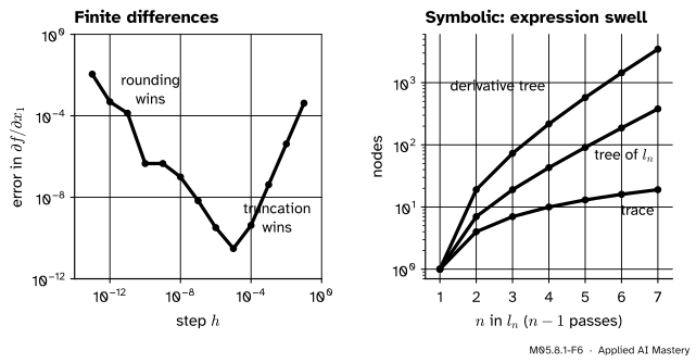
Why not just use finite differences? The central difference of M05.2.4 approximates each partial derivative with two runs of \(f\), so a gradient in \(n\) inputs costs \(2n\) runs. For a network with a million weights that is two million runs of the network for one training step. The answer is also inexact: the error falls like \(h^2\) until rounding takes over, and then grows again (M04.2.4).
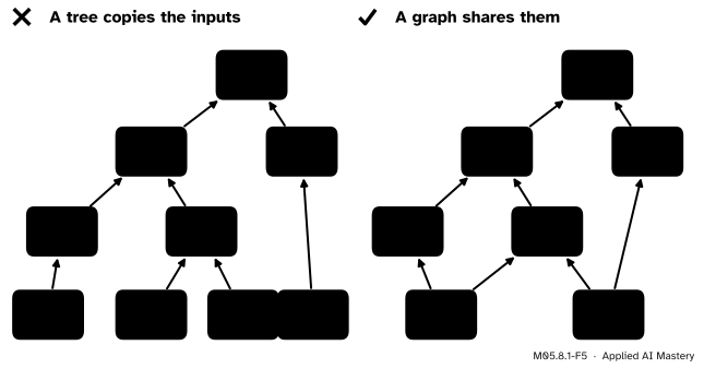
Why not symbolic differentiation? A computer algebra system applies the rules of differentiation to the formula itself. But a formula written out in full is a tree, not a graph: a shared subexpression is copied every time it is used. The logistic map \({l_{k+1} = 4\,l_k(1 - l_k)}\), started from \({l_1 = x}\), uses \(l_k\) twice, so the tree of \(l_n\) doubles with each pass, and the product rule copies each factor again into the derivative. This blow-up is called expression swell.
M05.8.1-F6
Left: a finite difference is either truncated (large \(h\)) or swamped by rounding (small \(h\)). Right: written as trees, the logistic map and above all its derivative swell; the trace grows by three steps per pass.
Automatic differentiation avoids both troubles. It works on the trace, where every shared value is stored once, and it applies the exact derivative of each elementary step, so there is no step size \(h\) and no truncation.
Worked example
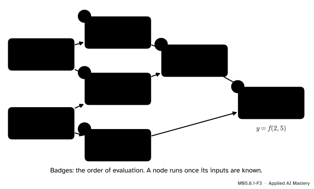
The running program at (2, 5). Go down the trace, filling in numbers:
\({v_{-1} = 2}\) and \({v_0 = 5}\).
\({v_1 = \ln 2 \approx 0.693}\).
\({v_2 = 2 \times 5 = 10}\).
\({v_3 = \sin 5 \approx -0.959}\) (5 radians lies in the fourth quarter of the circle).
The worked trace. The badges give one topological order; the order 3, 1, 2, 4, 5 would do as well, but \(v_4\) can never come before \(v_1\) or \(v_2\).
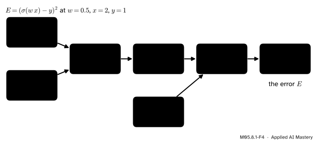
The running chain of M04.3.4. A classifier with weight \({w = 0.5}\) scores the input \({x = 2}\), turns the score into a probability, and pays the squared error against the target \({y = 1}\). Treat \(w\) as the only input, and \(x\) and \(y\) as fixed numbers:
\({v_0 = w = 0.5}\).
\({v_1 = v_0 \cdot 2 = 1}\).
\({v_2 = \sigma(v_1) \approx 0.731}\).
\({v_3 = v_2 - 1 \approx -0.269}\).
\({v_4 = v_3^2 \approx 0.072}\).
M05.8.1-F4
The running chain as a graph. It is a straight line because every value is used once: the simplest kind of computational graph, and the shape of every layer-by-layer network.
This is the forward pass that lesson M04.3.4 ran before multiplying local slopes backwards. The only new idea is to see it as a graph, because the same backward walk works on any graph, not only on a chain (M05.8.3).
Code
From scratch: a program stored as a list of nodes, deliberately out of order. Each node names its operation and its inputs. A topological sort puts the list in order, and evaluation walks along it.
import mathOPS = {"add": lambda a, b: a + b, "sub": lambda a, b: a - b, "mul": lambda a, b: a * b,"ln": math.log, "sin": math.sin, "exp": math.exp, "tanh": math.tanh,"sigmoid": lambda z: 1/ (1+ math.exp(-z)), "square": lambda a: a * a,}# (name, operation, inputs); an input is the name of a node or a plain numberPROGRAM = [ ("v5", "sub", ["v4", "v3"]), ("v2", "mul", ["x1", "x2"]), ("v4", "add", ["v1", "v2"]), ("v1", "ln", ["x1"]), ("v3", "sin", ["x2"]),]def topological_order(program, inputs):"""Kahn's algorithm: repeatedly take a node whose parents are all known.""" known, order, waiting =set(inputs), [], list(program)while waiting: ready = [node for node in waitingifall(isinstance(a, float) or a in known for a in node[2])]ifnot ready:raiseValueError("the graph has a cycle or a missing input")for node in ready: order.append(node) known.add(node[0]) waiting.remove(node)return orderdef evaluate(program, inputs): values =dict(inputs)for name, op, args in topological_order(program, inputs): values[name] = OPS[op](*[a ifisinstance(a, float) else values[a] for a in args])return valuesvalues = evaluate(PROGRAM, {"x1": 2.0, "x2": 5.0})print([name for name, _, _ in topological_order(PROGRAM, ["x1", "x2"])])print({k: round(v, 3) for k, v in values.items()})
A loop unrolls when we record what actually runs. The recorder below runs the program of the second figure and writes one node for each elementary step it performs:
def record_logistic(x, passes=3): trace, l = [], "x"for k inrange(1, passes +1): # p{k} is the value after pass k trace += [(f"a{k}", "mul", [4.0, l]), (f"b{k}", "sub", [1.0, l]), (f"p{k}", "mul", [f"a{k}", f"b{k}"])] l =f"p{k}" last = evaluate(trace, {"x": x})[l] trace.append(("y", "square", [l]) if last >0.5else ("y", "sub", [1.0, l]))return tracefor x in (0.2, 0.3): trace = record_logistic(x) out = evaluate(trace, {"x": x})print(f"x = {x}: {len(trace)} steps, after pass 3 {out['p3']:.4f}, last step {trace[-1][1]}, y = {out['y']:.4f}")
x = 0.2: 10 steps, after pass 3 0.2890, last step sub, y = 0.7110
x = 0.3: 10 steps, after pass 3 0.9943, last step square, y = 0.9887
Last, the two alternatives. Finite differences: count the runs a central-difference gradient needs. Symbolic differentiation: build the logistic map as a tree, differentiate it by the sum and product rules alone, and count nodes.
runs =0def f(x):global runs runs +=1return math.log(x[0]) + x[0] * x[1] - math.sin(x[1])def central_gradient(f, x, h=1e-5): grad = []for i inrange(len(x)): up, down =list(x), list(x) up[i] += h down[i] -= h grad.append((f(up) - f(down)) / (2* h))return gradprint("central-difference gradient:", [round(g, 6) for g in central_gradient(f, [2.0, 5.0])], "runs:", runs)def tree(n): # l_1 = x, l_(k+1) = 4 l_k (1 - l_k), with no sharing t = ("x",)for _ inrange(n -1): t = ("*", ("*", ("c", 4), t), ("-", ("c", 1), t))return tdef d(t): # the sum and product rules, nothing elseif t[0] =="x":return ("c", 1)if t[0] =="c":return ("c", 0) a, b = t[1], t[2]if t[0] in"+-":return (t[0], d(a), d(b))return ("+", ("*", d(a), b), ("*", a, d(b)))def size(t):return1if t[0] in"xc"else1+ size(t[1]) + size(t[2])for n inrange(1, 8):print(f"n = {n}: tree of l_n {size(tree(n)):4d} nodes, its derivative {size(d(tree(n))):5d}, "f"trace {1+3* (n -1):3d}")
central-difference gradient: [5.5, 1.716338] runs: 4
n = 1: tree of l_n    1 nodes, its derivative     1, trace   1
n = 2: tree of l_n    7 nodes, its derivative    19, trace   4
n = 3: tree of l_n   19 nodes, its derivative    73, trace   7
n = 4: tree of l_n   43 nodes, its derivative   217, trace  10
n = 5: tree of l_n   91 nodes, its derivative   577, trace  13
n = 6: tree of l_n  187 nodes, its derivative  1441, trace  16
n = 7: tree of l_n  379 nodes, its derivative  3457, trace  19
The tree of \(l_n\) has \({3 \cdot 2^n - 5}\) nodes for every \({n \ge 1}\), doubling with each pass, and its naive derivative grows faster still, while the trace grows by three steps a pass. Real algebra systems simplify as they go, which helps, but the tree form is the root of the trouble.
Explore
This module’s interactive, the graph stepper, lives in lesson M05.8.3. For now, choose its reverse mode and press Step seven times: that is the forward pass alone, each node getting its value once its parents are known. Move the sliders for \(x_1\) and \(x_2\) and every value follows.
Pitfalls
M05.8.1-F5
Wrong beside right. A formula read as a tree copies every input it uses twice. The computational graph keeps one node per value and lets its arrows fan out.
“A computational graph is the same as the formula’s expression tree.”
A tree gives every use of a value its own copy, so shared work is repeated and grows exponentially, as with the logistic map. The graph stores each value once. When derivatives later flow back through the graph, the two arrows out of \(x_1\) carry two contributions that must be added; in a tree they would sit on two separate leaves and could be missed.
“Automatic differentiation is a clever finite difference.”
It never chooses a step \(h\) and never subtracts two nearly equal values of \(f\). It applies the exact derivative of each elementary step to the numbers in the trace, so its answer is exact up to the rounding of ordinary arithmetic, the same rounding that computing \(f\) itself suffers.
“Programs with loops and if-statements cannot be differentiated automatically.”
They can: a run leaves a trace with the loop unrolled and only the branch taken. What a trace cannot give is a slope at an input where a branch switches and the function jumps; there the function has no slope to give.
Check yourself
Recall
1. What is an evaluation trace, or Wengert list?
Show answer
The list of intermediate variables \(v_i\) that a program computes, one elementary operation per line, with every line using only inputs and earlier lines.
2. Why is a computational graph acyclic?
Show answer
Every edge runs from a variable to one with a larger index, so along any path the index rises and can never return to its starting value.
3. What is \(f(2, 5)\) for \({f(x_1, x_2) = \ln x_1 + x_1 x_2 - \sin x_2}\), and which value of the trace is \({\sin 5}\)?
Show answer
About 11.652. \({\sin 5 \approx -0.959}\) is \(v_3\).
4. How many runs of \(f\) does a central-difference gradient in \(n\) inputs need?
Show answer
\(2n\): one on each side of the point for each input.
5. What is expression swell?
Show answer
The blow-up in size of a formula and of its symbolic derivative when shared subexpressions are copied at every use, as the product rule does; the tree of the logistic map doubles with each pass.
Exercises
1.★ Write the evaluation trace of \({g(x_1, x_2) = e^{x_1 x_2} + x_2}\) and evaluate it at \({(1, 2)}\).
Show solution
\({v_{-1} = x_1 = 1}\), \({v_0 = x_2 = 2}\), \({v_1 = v_{-1} v_0 = 2}\), \({v_2 = \exp v_1 = e^2 \approx 7.389}\), \({v_3 = v_2 + v_0 \approx 9.389}\). So \({g(1, 2) = e^2 + 2 \approx 9.389}\). The input \(v_0\) is used twice, so its node has two arrows out.
2.★★ The single-example log loss of logistic regression is \({E = -\ln \sigma(w x + b)}\) for a positive example. Write its trace with inputs \(w\) and \(b\), the fixed input \({x = 2}\), and evaluate it at \({w = 0.5}\), \({b = 0}\). Which node would change if the example were negative, with loss \({-\ln(1 - \sigma(wx + b))}\)?
Show solution
\({v_{-1} = w = 0.5}\), \({v_0 = b = 0}\), \({v_1 = 2 v_{-1} = 1}\), \({v_2 = v_1 + v_0 = 1}\), \({v_3 = \sigma(v_2) \approx 0.731}\), \({v_4 = \ln v_3 \approx -0.313}\), \({v_5 = -v_4 \approx 0.313}\). For a negative example a new node \({1 - v_3}\) sits between \(v_3\) and the logarithm; the rest of the graph is unchanged. In code, an if on the label chooses which trace is recorded.
3.★★★ The expression tree of \(l_n\) has \(T_n\) nodes, with \({T_1 = 1}\). Show that \({T_{n+1} = 2T_n + 5}\) and hence \({T_n = 3 \cdot 2^n - 5}\) for \({n \ge 1}\). How many nodes does the trace of \(l_n\) have?
Show solution
The tree of \(l_{n+1}\), the product of \({4\,l_n}\) and \({1 - l_n}\), has a root \(\times\), an inner \(\times\) with the constant 4, a \(-\) with the constant 1, and two copies of the tree of \(l_n\): five new nodes and \(2T_n\) copied ones, so \({T_{n+1} = 2T_n + 5}\). Check the formula: \({3 \cdot 2 - 5 = 1 = T_1}\), and if \({T_n = 3 \cdot 2^n - 5}\) then
By induction the formula holds for every \(n\). The trace stores \(l_n\) once, so each pass adds three steps: \({1 + 3(n - 1)}\) nodes, counting the input. Linear against exponential.
Summary card
A program is a graph of elementary steps.
M05.8.1-F1
One line of the trace, one node of the graph.
Trace: \({v_i = \varphi_i(\text{parents})}\), each parent earlier in the list.
Graph: a DAG; evaluate it in any topological order.
Running program: \({f(2, 5) \approx 11.652}\).
Finite differences cost \(2n\) runs and are inexact; symbolic trees swell.
Sources and next steps
Sources. Each was opened and checked against this lesson on 15 November 2026.
A. G. Baydin, B. A. Pearlmutter, A. A. Radul and J. M. Siskind, Automatic Differentiation in Machine Learning: a Survey, JMLR 18(153), 2018. Section 2.1: a gradient by finite differences costs \(O(n)\) evaluations, and a Jacobian \(2mn\) when each output is counted separately; section 2.2 and Table 1: expression swell on the logistic map \({l_{n+1} = 4l_n(1 - l_n)}\); section 3: the evaluation trace, called a Wengert list, with inputs numbered from \({v_{1-n}}\), Figure 4 (the graph of the running program) and Table 2 (its primal trace at \({(2, 5)}\), \({y = 11.652}\)); and the remark that a trace records only the control-flow path taken.
P. Bright, A. Edelman and S. G. Johnson, Matrix Calculus (for Machine Learning and Beyond), notes for MIT course 18.S096. Section 8.2 shows naive symbolic differentiation of a simple iteration swelling; section 8.3 builds automatic differentiation on computational graphs.
M. P. Deisenroth, A. A. Faisal and C. S. Ong, Mathematics for Machine Learning, section 5.6.2: Example 5.14 breaks a function into intermediate variables with a computation graph (Figure 5.11), and equation (5.143) writes a graph as \({x_i = g_i(x_{\text{Pa}(x_i)})}\).