A derivative in matrix calculus is a block of numbers with a definite shape. Learn the three kinds (gradient, Jacobian, gradient by a matrix), the two layout conventions, and derive the first identities in index notation.
M05.7.1L2 Intermediate25 minIn review (what this means)
The maths and code on this page are checked by automated tests on every change, but an independent reader has not signed it off yet. Spot a mistake or a confusing step? Tell us.
Give the shape of a gradient, a Jacobian and a gradient with respect to a matrix before computing any entry.
Translate a formula between numerator layout and denominator layout by transposing.
Derive the gradients of a-transpose x, x-transpose A x, the squared norm and the squared residual norm in index notation, and the Jacobian of A x.
Check any gradient identity with central differences on random matrices, asserting shapes first.
The question
Two well-known books give the derivative of \(\mat{A}\vect{x}\) with respect to \(\vect{x}\). One says it is \(\mat{A}\), the other says \(\mat{A}\T\). Both books are correct. How can that be, and how do you keep the shapes straight, so that a gradient you derive by hand can actually be subtracted from the weights it belongs to?
Intuition
A derivative is not just a number once there are many inputs or many outputs. It is a block of numbers, one for each pair (output, input), and the block has a shape. Before computing any entry, you can say what that shape must be.
M05.7.1-F1
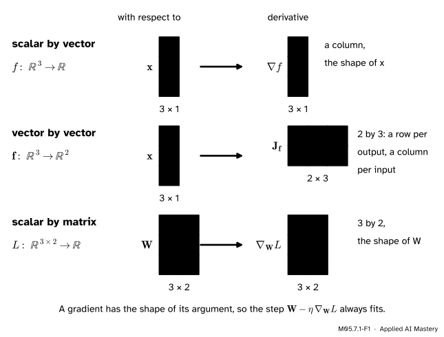
The three kinds of derivative in this module, drawn as blocks. A scalar differentiated by a vector gives a column like the vector; a vector of \(m\) outputs differentiated by \(n\) inputs gives an \(m\) by \(n\) Jacobian; a scalar differentiated by a matrix gives a matrix of the same shape.
Three rules of thumb come out of the picture. A gradient has the shape of the thing you differentiate with respect to, so a weight update \({\mat{W} - \eta\,\nabla_{\mat{W}} L}\) always makes sense. A Jacobian has one row for each output and one column for each input. And whatever convention a book uses, the entries are always the same partial derivatives: only their arrangement can differ.
Build it up
Step 1. Scalar by vector. For \(f : \R^n \to \R\), the gradient collects the \(n\) partial derivatives \(\pd{f}{x_i}\) in a column, exactly as in M05.2: \(\nabla f(\vect{x})\) has shape \({n \times 1}\), like \(\vect{x}\).
Step 2. Vector by vector. For \(\vect{f} : \R^n \to \R^m\) there are \({m \cdot n}\) partial derivatives \(\pd{f_i}{x_j}\). The Jacobian \(\mat{J}_{\vect{f}}\) of M05.4 puts the one for output \(i\) and input \(j\) in row \(i\), column \(j\). Row \(i\) is the transposed gradient of \(f_i\).
Step 3. Scalar by matrix. For a loss \(L\) of a weight matrix \(\mat{W}\) with \(d\) rows and \(m\) columns, there are \({d \cdot m}\) partial derivatives \(\pd{L}{w_{ij}}\). We place each one where its weight sits, so \(\nabla_{\mat{W}} L\) is a \(d\) by \(m\) matrix. Entry \((i, j)\) says how fast the loss changes when weight \(w_{ij}\) alone is nudged.
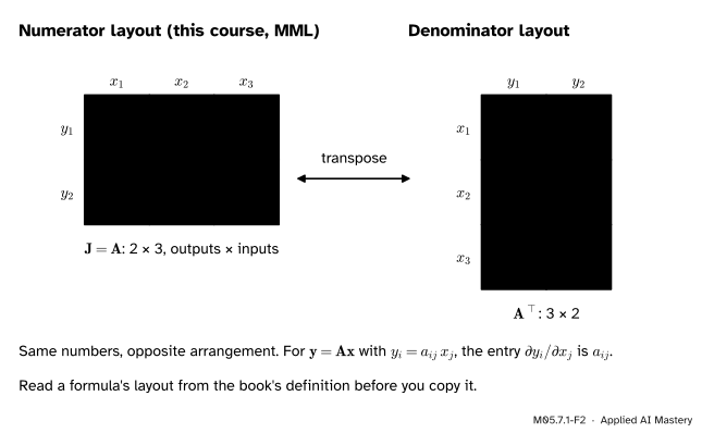
Step 4. Two layouts. Step 2 is the numerator layout: the outputs (the numerator of \(\partial f_i / \partial x_j\)) index the rows. The denominator layout lets the inputs index the rows instead, and so gives the transpose.
M05.7.1-F2
The derivative of \(\vect{y} = \mat{A}\vect{x}\) for a 2 by 3 matrix \(\mat{A}\), in both layouts. The six numbers are the same; one layout is the transpose of the other.
That settles the opening question. A book in numerator layout writes the derivative of \(\mat{A}\vect{x}\) as \(\mat{A}\); a book in denominator layout writes \(\mat{A}\T\). This course uses numerator layout for Jacobians, like Mathematics for Machine Learning (MML). There is one twist: MML writes the gradient of a scalar function as a row, the \({1 \times n}\) Jacobian, while this course writes it as a column with the shape of \(\vect{x}\). So our gradient is the transpose of MML’s. Their identity (5.107) and ours read
NoteDefinitions: the three derivatives and their shapes
For \(f : \R^n \to \R\), the gradient\(\nabla f(\vect{x})\) is the \({n \times 1}\) column with entries \(\pd{f}{x_i}\).
For \(\vect{f} : \R^n \to \R^m\), the Jacobian\(\mat{J}_{\vect{f}}(\vect{x})\) is the \({m \times n}\) matrix with entry \((i, j)\) equal to \(\pd{f_i}{x_j}\) (numerator layout). For scalar \(f\) it is the row \(\nabla f\T\).
For \(L : \R^{d \times m} \to \R\), the gradient with respect to the matrix\(\nabla_{\mat{W}} L\) is the \({d \times m}\) matrix with entry \((i, j)\) equal to \(\pd{L}{w_{ij}}\).
Every identity below is derived in index notation, as in M03.10.2: a repeated index is summed, and the rate of change of \(x_i\) when \(x_k\) moves is \(\pd{x_i}{x_k} = \delta_{ik}\).
Identity 1: a linear function. Let \(f = \vect{a}\T\vect{x} = a_i x_i\). Then
Identity 2: a quadratic form. Let \(f = \vect{x}\T\mat{A}\vect{x} = x_i\, a_{ij}\, x_j\) for any square \(\mat{A}\). The product rule gives two terms, one for each factor that contains \(\vect{x}\):
So \(\nabla(\vect{x}\T\mat{A}\vect{x}) = {(\mat{A} + \mat{A}\T)\vect{x}}\). When \(\mat{S}\) is symmetric, \(\mat{S}\T = \mat{S}\) and the gradient is \(2\mat{S}\vect{x}\).
Identity 3: the squared norm.\(\norm{\vect{x}}^2 = \vect{x}\T\mat{I}\vect{x}\), and \(\mat{I}\) is symmetric, so Identity 2 gives \(\nabla\norm{\vect{x}}^2 = 2\vect{x}\).
Identity 4: the Jacobian of a linear map. For \(\vect{y} = \mat{A}\vect{x}\) with \(\mat{A}\) of shape \({m \times n}\), \(y_i = a_{ij}\, x_j\), so
Identity 5: the squared residual. Let \(f = \norm{\mat{A}\vect{x} - \vect{b}}^2\) and call the residual \(\vect{r} = \mat{A}\vect{x} - \vect{b}\), so \(f = r_i\, r_i\). Each \(r_i\) depends on \(\vect{x}\) through \(r_i = a_{ij} x_j - b_i\), with \(\pd{r_i}{x_k} = a_{ik}\) by Identity 4. Then
The shapes confirm it: \(\mat{A}\T\) is \({n \times m}\) and \(\vect{r}\) is \({m \times 1}\), so the product is \({n \times 1}\), the shape of \(\vect{x}\).
M05.7.1-F5
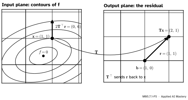
Why \(\mat{A}\T\) appears in Identity 5, for \(\mat{T}\) with rows \((1, 1)\) and \((-1, 2)\) and \(\vect{b} = (1, 0)\). The residual \(\vect{r}\) lives among the outputs; \(\mat{T}\T\) carries it back among the inputs, where \(2\mat{T}\T\vect{r}\) is the gradient, across the contour of \(f\).
Go deeper: Identity 5 as a product of Jacobians
Write \(f = g(\vect{h}(\vect{x}))\) with \(\vect{h}(\vect{x}) = \mat{A}\vect{x} - \vect{b}\) and \(g(\vect{r}) = \vect{r}\T\vect{r}\). By Identity 4, \(\mat{J}_{\vect{h}} = \mat{A}\); by Identity 3 and the remark that a scalar’s Jacobian is its transposed gradient, \(\mat{J}_g = 2\vect{r}\T\). The chain rule of M05.4.3 multiplies Jacobians, so \(\mat{J}_f = 2\vect{r}\T\mat{A}\), a \({1 \times n}\) row. Its transpose is the gradient, \(2\mat{A}\T\vect{r}\). The transpose in Identity 5 is the price of writing gradients as columns.
Worked example
The running bowl. The bowl \(f(x, y) = x^2 + 2y^2\) is the quadratic form \(\vect{x}\T\mat{S}\vect{x}\) with \(\mat{S} = \operatorname{diag}(1, 2)\), because \({x \cdot 1 \cdot x} + {y \cdot 2 \cdot y} = x^2 + 2y^2\). \(\mat{S}\) is symmetric, so Identity 2 gives
\[
\nabla f = 2\mat{S}\vect{x} = (2x,\; 4y),
\]
which is \((2, 4)\) at \((1, 1)\), as M04.10 found one partial derivative at a time.
A squared residual. Take the running map \(\mat{T}\), rows \((1, 1)\) and \((-1, 2)\), the target \(\vect{b} = (1, 0)\) and the point \(\vect{x} = (1, 1)\). Follow Identity 5 one block at a time.
M05.7.1-F3
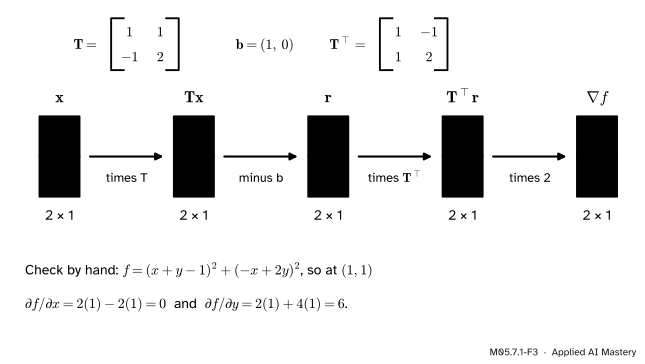
The worked example as a chain of blocks. Every block is \({2 \times 1}\), the shape of \(\vect{x}\), so the gradient can be subtracted from \(\vect{x}\) directly.
First \(\mat{T}\vect{x} = (1 + 1,\; -1 + 2) = (2, 1)\). The residual is \(\vect{r} = (2, 1) - (1, 0) = (1, 1)\), so \(f = 1 + 1 = 2\). Then
at \((1, 1)\). The identity agrees. The zero says that moving \(x\) alone does not change \(f\) to first order here: the contour through \((1, 1)\) is flat in that direction, as the figure in the formal section shows.
Code
From scratch: a gradient and a Jacobian by central differences, then every identity of the formal section checked on random matrices with a fixed seed. Shapes are asserted before values.
import numpy as npdef num_grad(f, x, h=1e-6):"""Central differences in each coordinate: a gradient with the shape of x.""" g = np.zeros_like(x, dtype=float)for i inrange(x.size): e = np.zeros_like(x, dtype=float) e.flat[i] = h g.flat[i] = (f(x + e) - f(x - e)) / (2* h)return gdef num_jac(F, x, h=1e-6):"""Central differences, one input at a time: column j of the Jacobian is dF/dx_j.""" cols = []for j inrange(x.size): e = np.zeros_like(x, dtype=float) e[j] = h cols.append((F(x + e) - F(x - e)) / (2* h))return np.column_stack(cols)rng = np.random.default_rng(7)n, m =4, 3x, a = rng.normal(size=n), rng.normal(size=n)A = rng.normal(size=(n, n)) # square, not symmetricS = A + A.T # symmetricM, b = rng.normal(size=(m, n)), rng.normal(size=m)identities = {"a^T x": (lambda v: a @ v, a),"x^T A x": (lambda v: v @ A @ v, (A + A.T) @ x),"x^T S x": (lambda v: v @ S @ v, 2* S @ x),"||x||^2": (lambda v: v @ v, 2* x),"||Mx - b||^2": (lambda v: np.sum((M @ v - b) **2), 2* M.T @ (M @ x - b)),}gaps = {}for name, (f, formula) in identities.items(): numeric = num_grad(f, x)assert numeric.shape == formula.shape == x.shape gaps[name] = np.abs(numeric - formula).max()print(f"{name:13s} shape {formula.shape} largest gap {gaps[name]:.1e}")J = num_jac(lambda v: M @ v, x)print("Jacobian of Mx: shape", J.shape, " largest gap from M:", f"{np.abs(J - M).max():.1e}")
a^T x         shape (4,)   largest gap 1.1e-10
x^T A x       shape (4,)   largest gap 7.6e-11
x^T S x       shape (4,)   largest gap 1.5e-10
||x||^2       shape (4,)   largest gap 3.7e-11
||Mx - b||^2  shape (4,)   largest gap 2.3e-10
Jacobian of Mx: shape (3, 4)   largest gap from M: 7.4e-11
The gaps are tiny, about the size of the rounding error of a central difference. The worked example, with the same functions:
bowl gradient at (1, 1): [2. 4.]
residual: [1. 1.]   gradient 2 T^T r: [0. 6.]
by differences: [0. 6.]
SciPy’s scipy.optimize.approx_fprime does the same with forward differences. For a function with \(m\) outputs it returns an \({m \times n}\) array: the Jacobian in numerator layout.
from scipy.optimize import approx_fprimeJ_scipy = approx_fprime(x, lambda v: M @ v)g_scipy = approx_fprime(x, lambda v: v @ A @ v)print("approx_fprime shapes:", J_scipy.shape, g_scipy.shape)print("largest gaps:", f"{np.abs(J_scipy - M).max():.1e}", f"{np.abs(g_scipy - (A + A.T) @ x).max():.1e}")
approx_fprime shapes: (3, 4) (4,)
largest gaps: 1.3e-08 3.6e-08
Forward differences are less accurate than central ones (their error shrinks like \(h\), not \(h^2\)), so the gaps are larger, but still small.
Explore
The gradient heatmap of M05.7.2 shows a gradient with respect to a matrix as a grid with the shape of the matrix. Pick the preset \(\vect{a}\T\mat{X}\vect{b}\) and switch to the common mistake: the shapes no longer match, and the read-out says so.
Pitfalls
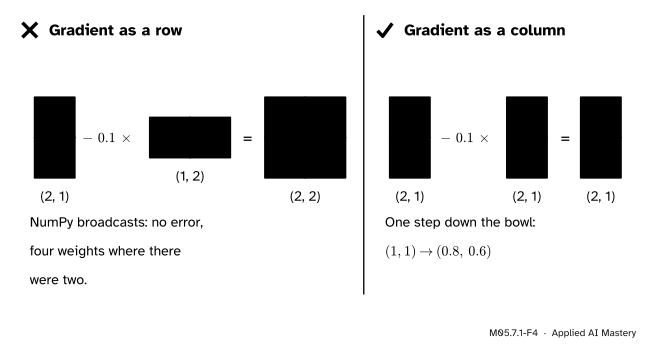
M05.7.1-F4
Wrong beside right: one gradient step on the running bowl from \((1, 1)\) with \(\eta = 0.1\). With the gradient written as a row, NumPy broadcasts the subtraction into a 2 by 2 array without complaint.
“A row gradient and a column gradient are the same thing.”
They hold the same numbers, but code does not forgive the difference. Subtracting an array of shape (1, 2) from one of shape (2, 1) broadcasts to shape (2, 2), as in the figure, and training goes on with nonsense. Keep gradients in the shape of their argument, and assert shapes.
“The gradient of \(\vect{x}\T\mat{A}\vect{x}\) is \(2\mat{A}\vect{x}\).”
Only when \(\mat{A}\) is symmetric. In general it is \({(\mat{A} + \mat{A}\T)\vect{x}}\) (Identity 2). The code above asserts that \(2\mat{A}\vect{x}\) differs from the true gradient for its random, non-symmetric \(\mat{A}\).
“I can copy an identity from any book.”
Check the book’s layout first. A formula from a denominator-layout source is the transpose of ours, and a source that writes gradients as rows (as MML does) gives the transpose of our column. If the shape of the copied formula does not match the shape of the argument, it was written in the other layout.
Check yourself
Recall
1. What is the shape of the Jacobian of \(\vect{f} : \R^5 \to \R^3\) in numerator layout?
Show answer
\({3 \times 5}\): one row for each output, one column for each input.
2. A loss depends on a weight matrix of shape \({10 \times 4}\). What is the shape of its gradient?
Show answer
\({10 \times 4}\), the shape of the weight matrix.
3. What is the gradient of \(\vect{a}\T\vect{x}\)?
Show answer
\(\vect{a}\).
4. What is the gradient of \(\norm{\mat{A}\vect{x} - \vect{b}}^2\)?
Show answer
\(2\mat{A}\T(\mat{A}\vect{x} - \vect{b})\).
5. How are the numerator and the denominator layout related?
Show answer
Each is the transpose of the other. The entries are the same partial derivatives.
Exercises
1.★ State the shapes of: the gradient of \(f : \R^{7} \to \R\); the Jacobian of \(\vect{x} \mapsto \mat{A}\vect{x}\) for \(\mat{A}\) of shape \({2 \times 7}\); the gradient of a loss with respect to a bias vector in \(\R^{16}\).
Show solution
\({7 \times 1}\), the shape of the input. \({2 \times 7}\), and the Jacobian is \(\mat{A}\) itself by Identity 4. \({16 \times 1}\), the shape of the bias.
2.★★ Find the gradient of \(f(\vect{x}) = \vect{x}\T\mat{A}\vect{x}\) for \(\mat{A}\) with rows \((1, 4)\) and \((0, 1)\) at \(\vect{x} = (1, 0)\). Check it by expanding \(f\).
Show solution
\(\mat{A} + \mat{A}\T\) has rows \((2, 4)\) and \((4, 2)\), so the gradient is \({(\mat{A} + \mat{A}\T)\vect{x}} = (2, 4)\). Expanding, \(f = x^2 + 4xy + y^2\), so \(\pd{f}{x} = 2x + 4y = 2\) and \(\pd{f}{y} = 4x + 2y = 4\) at \((1, 0)\). The shortcut \(2\mat{A}\vect{x}\) would give \((2, 0)\), which is wrong.
3.★★★ Derive in index notation the gradient of the weighted squared residual \(f(\vect{x}) = (\mat{A}\vect{x} - \vect{b})\T\mat{D}(\mat{A}\vect{x} - \vect{b})\), where \(\mat{D}\) is a symmetric \({m \times m}\) matrix, and check the shape.
Show solution
With \(\vect{r} = \mat{A}\vect{x} - \vect{b}\), \(f = r_i\, d_{ij}\, r_j\) and \(\pd{r_i}{x_k} = a_{ik}\). The product rule gives
For symmetric \(\mat{D}\) the two terms are equal, so \(\nabla f = 2\mat{A}\T\mat{D}(\mat{A}\vect{x} - \vect{b})\). Shapes: \({(n \times m)(m \times m)(m \times 1)}\) is \({n \times 1}\), like \(\vect{x}\). With \(\mat{D} = \mat{I}\) this is Identity 5.
Summary card
A derivative is a block with a definite shape.
M05.7.1-F1
Gradient, Jacobian, gradient by a matrix.
Shapes:\(\nabla f\) like \(\vect{x}\); \(\mat{J}\) is outputs by inputs; \(\nabla_{\mat{W}} L\) like \(\mat{W}\).
Linear:\(\nabla(\vect{a}\T\vect{x}) = \vect{a}\), and the Jacobian of \(\mat{A}\vect{x}\) is \(\mat{A}\).
Sources. Each was opened and checked against this lesson on 15 November 2026.
Marc Peter Deisenroth, A. Aldo Faisal and Cheng Soon Ong, Mathematics for Machine Learning, Section 5.2, equation (5.40): the gradient as a \({1 \times n}\) row; Section 5.3, (5.58) and the remark that follows it: the \({m \times n}\) Jacobian, numerator layout, and the denominator layout as its transpose; Section 5.5, (5.104) to (5.107), the identities for \(\vect{x}\T\vect{a}\), \(\vect{a}\T\vect{x}\) and \(\vect{x}\T\mat{B}\vect{x}\) in row form.
Paige Bright, Alan Edelman and Steven G. Johnson, Matrix Calculus (for Machine Learning and Beyond), course notes of MIT 18.S096: Example 10 in Section 2.3 (\(\nabla(\vect{x}\T\mat{A}\vect{x}) = {(\mat{A} + \mat{A}\T)\vect{x}}\), and \(2\mat{A}\vect{x}\) for symmetric \(\mat{A}\) in Example 13) and Example 11 in Section 2.4 (the linear map \(\mat{A}\) is its own Jacobian).
Kaare Brandt Petersen and Michael Syskind Pedersen, The Matrix Cookbook, version of 15 November 2012, Section 2.4.1, (69); Section 2.4.2, (81); and Section 2.6.1, (131).
SciPy reference, scipy.optimize.approx_fprime: forward differences, and an \((m, n)\) Jacobian for a function with \(m\) outputs.