Normals, tangent planes and the distance to a boundary
The gradient sticks straight out of a level surface, so it gives the tangent plane at once. Dividing by its length gives the distance to a level set to first order, exactly for a linear classifier’s boundary, and the smallest input change that moves a score, the idea behind the fast gradient sign attack.
M05.3.4L2 Intermediate25 minIn review (what this means)
The maths and code on this page are checked by automated tests on every change, but an independent reader has not signed it off yet. Spot a mistake or a confusing step? Tell us.
Use the gradient as a normal vector to write the tangent plane to a level surface.
Derive the first-order distance from a point to a level set, the gap in value divided by the length of the gradient, and say when it is exact.
Compute the distance from a point to a hyperplane and read it as the margin of a linear classifier.
Find the smallest change of an input that moves a linear score, in the L2 norm and in the max-norm, and recognise the fast gradient sign attack.
Compare the first-order distance with the exact distance found by scipy.optimize.minimize.
The question
A classifier draws a boundary through its input space: one side is “spam”, the other is not. How far is a given email from that boundary, and what is the smallest change to its features that would carry it across? Both are questions about the distance from a point to a level set, and the gradient answers them, exactly for a linear score and to first order for any other.
From the last lesson
1. What is the steepest-descent step in the max-norm?
Show answer
\({-\operatorname{sign}(\nabla f)}\): every coordinate moves by the full amount against the sign of its partial derivative.
2. For \({\nabla f = (2, 4)}\), what is the steepest-descent step in the L1 norm?
Show answer
\({(0, -1)}\): only the coordinate with the larger partial derivative moves.
Intuition
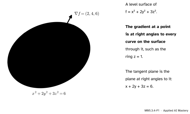
Lesson 2 showed that the gradient is at right angles to every curve inside a level set. In three dimensions a level set is a surface, and an arrow at right angles to every curve on it sticks straight out of it: a normal. The flat plane at right angles to that arrow just touches the surface: the tangent plane.
M05.3.4-F1
A level surface of \({f = x^2 + 2y^2 + 3z^2}\). The gradient at \({(1, 1, 1)}\) is a normal to it, and the tangent plane is the plane at right angles to the gradient.
The same arrow measures distance. Its length is the steepest slope, so to change \(f\) by a given amount the shortest walk is along the gradient, and its length is about the change divided by \({\norm{\nabla f}}\). That turns “how far to the boundary?” into one division.
Build it up
Step 1. The tangent plane. A point \(\vect{x}\) lies in the plane through \(\vect{a}\) at right angles to \({\nabla f(\vect{a})}\) exactly when the step \({\vect{x} - \vect{a}}\) is perpendicular to the gradient: \({\nabla f(\vect{a})\T(\vect{x} - \vect{a})} = {0}\). In the plane this is the tangent line to a contour; in space it is a plane; in \(\R^n\) it is a hyperplane.
Step 2. Replace \(f\) by its linear model. Near \(\vect{x}\), lesson 1 gives \({f(\vect{x} + \vect{h})} \approx {f(\vect{x}) + \nabla f(\vect{x})\T\vect{h}}\). To reach the level \({f = c}\) the model needs \({\nabla f(\vect{x})\T\vect{h}} = {c - f(\vect{x})}\). Those steps fill a flat set parallel to the tangent plane, and by Cauchy-Schwarz the shortest of them has length
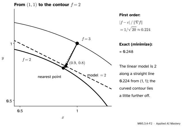
On the bowl from \({(1, 1)}\), where \({f = 3}\), to the contour \({f = 2}\): \({1/\sqrt{20} \approx 0.224}\). The true contour curves away from the model’s straight line, so the true distance, 0.248, is a little longer.
M05.3.4-F2
The linear model’s level set is a straight line \({1/\sqrt{20}}\) from \({(1, 1)}\). The real contour bends away from it, so the nearest point on it is a little further off.
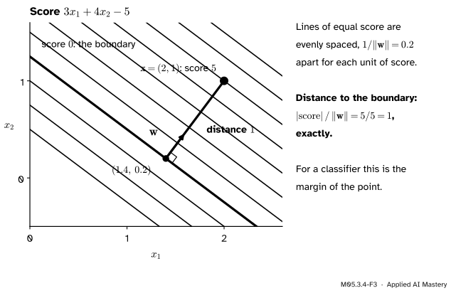
Step 3. A linear score is its own model. For \({f(\vect{x}) = \vect{w}\T\vect{x} + b}\) the gradient is \(\vect{w}\) everywhere and the linear model is \(f\) itself, so the formula is exact: the distance from \(\vect{x}\) to the hyperplane \({\vect{w}\T\vect{x} + b = 0}\) is \({\abs{\vect{w}\T\vect{x} + b}/\norm{\vect{w}}}\). With \({\vect{w} = (3, 4)}\), \({b = -5}\) and \({\vect{x} = (2, 1)}\) the score is \({6 + 4 - 5 = 5}\) and the distance is \({5/5 = 1}\).
M05.3.4-F3
For a linear score the level sets are evenly spaced parallel lines, \({1/\norm{\vect{w}}}\) apart per unit of score, and the first-order distance is the exact distance.
The formal statement
NoteResults: normal, tangent plane and distance
Let \(f\) be differentiable with \({\nabla f \neq \vect{0}}\) at the points involved.
\({\nabla f(\vect{a})}\) is normal to the level set through \(\vect{a}\), whose tangent plane is \({\nabla f(\vect{a})\T(\vect{x} - \vect{a})} = {0}\).
The distance from \(\vect{x}\) to the level set \({f = c}\) is, to first order, \({\abs{f(\vect{x}) - c}/\norm{\nabla f(\vect{x})}}\).
For \({f(\vect{x}) = \vect{w}\T\vect{x} + b}\) it is exact: the nearest point of the hyperplane is \({\vect{x} - \frac{f(\vect{x})}{\norm{\vect{w}}^2}\vect{w}}\).
Part 1 is lesson 2’s result read in space. For part 2, the step to the model’s level set must satisfy \({\nabla f\T\vect{h} = c - f(\vect{x})}\). By Cauchy-Schwarz,
so \({\norm{\vect{h}}} \ge {\abs{c - f(\vect{x})}/\norm{\nabla f}}\), with equality for \(\vect{h}\) along \({\pm\nabla f}\). “First order” means the estimate uses the linear model; for a smooth \(f\) the ratio of estimate to truth tends to 1 as \(\vect{x}\) approaches a point of the level set where the gradient is not \(\vect{0}\) (sketched below, measured in the code).
Go deeper: why the estimate and the true distance agree near the level set
Let \(\vect{q}\) be the nearest point of the level set to \(\vect{x}\), at distance \(\delta\). Along any curve in the level set through \(\vect{q}\) the squared distance to \(\vect{x}\) is smallest at \(\vect{q}\), so its slope there is 0: the step \({\vect{x} - \vect{q}}\) is perpendicular to every tangent direction of the level set, which makes it parallel to \({\nabla f(\vect{q})}\) (lesson 2). The linear model at \(\vect{q}\) then gives \({\abs{f(\vect{x}) - c}} = {\norm{\nabla f(\vect{q})}\,\delta}\) plus an error of order \({\delta^2}\). And \({\norm{\nabla f(\vect{x})}}\) differs from \({\norm{\nabla f(\vect{q})}}\) by order \(\delta\), since the gradient changes smoothly. Dividing, the estimate is \(\delta\) times a factor that differs from 1 by an amount of order \(\delta\), so the ratio tends to 1.
For part 3, put \({\vect{h}} = {-f(\vect{x})\,\vect{w}/\norm{\vect{w}}^2}\): then \({\vect{w}\T(\vect{x} + \vect{h}) + b} = {f(\vect{x}) - f(\vect{x})} = {0}\) and \({\norm{\vect{h}}} = {\abs{f(\vect{x})}/\norm{\vect{w}}}\). For a classifier with labels \({y = \pm 1}\) the signed version \({y\,(\vect{w}\T\vect{x} + b)/\norm{\vect{w}}}\) is the margin of the example, which support vector machines make large (ML02.7).
The smallest change that moves a score. Suppose we want to change a linear score by \(\Delta\) with the smallest step, measured by a ruler of lesson 3.
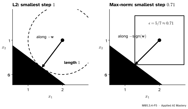
In L2 the step goes along \({\pm\vect{w}}\) and needs length \({\abs{\Delta}/\norm{\vect{w}}}\).
In the max-norm, a cube of half-width \(\epsilon\) can change the score by at most \({\epsilon\norm{\vect{w}}_1}\), at the corner \({\pm\epsilon\operatorname{sign}(\vect{w})}\) (lesson 3). So it needs \({\epsilon} = {\abs{\Delta}/\norm{\vect{w}}_1}\).
M05.3.4-F5
To reach the boundary from \({(2, 1)}\): a step of length 1 along \(-\vect{w}\) in L2, or a step of \({5/7 \approx 0.71}\) in every coordinate, along \({-\operatorname{sign}(\vect{w})}\), in the max-norm.
The fast gradient sign attack. Goodfellow, Shlens and Szegedy perturb an input \(\vect{x}\) of a network with loss \({J(\vect{x})}\) by \({\epsilon\operatorname{sign}(\nabla_{\vect{x}} J)}\): the steepest-ascent step of the loss in the max-norm, so every pixel moves by only \(\epsilon\). For logistic regression, \({p = \sigma(\vect{w}\T\vect{x} + b)}\) with the log loss, the chain rule of M05.2.3 gives
\[
\nabla_{\vect{x}} J = (p - y)\,\vect{w} ,
\]
so the attack is \({\vect{x} + \epsilon\operatorname{sign}(p - y)\operatorname{sign}(\vect{w})}\) and, the score being linear, it changes the score by exactly \({\epsilon\norm{\vect{w}}_1}\). In \(n\) dimensions \({\norm{\vect{w}}_1}\) grows like \(n\) when the weights have similar sizes, so many tiny changes add up to a large one: the paper’s linear explanation of adversarial examples.
Worked example
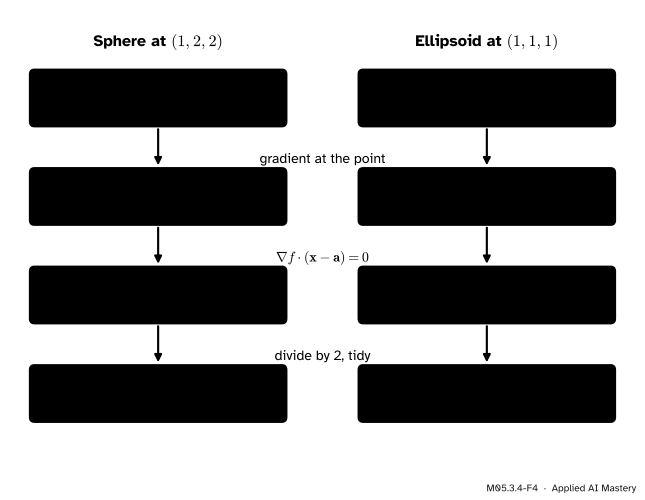
Tangent planes. For the sphere \({x^2 + y^2 + z^2 = 9}\) at \({(1, 2, 2)}\) the gradient is \({(2x, 2y, 2z) = (2, 4, 4)}\), so the plane is
Its normal \({(1, 2, 2)}\) is the radius, and its distance from the centre is \({9/\sqrt{1 + 4 + 4} = 3}\), the radius: a tangent plane to a sphere, as it should be. For the ellipsoid \({x^2 + 2y^2 + 3z^2 = 6}\) at \({(1, 1, 1)}\) the gradient is \({(2x, 4y, 6z) = (2, 4, 6)}\) and the plane is \({x + 2y + 3z = 6}\). Here the normal \({(1, 2, 3)}\) is not the radius \({(1, 1, 1)}\): they are \({22.2^\circ}\) apart.
M05.3.4-F4
Two tangent planes in three moves each: the gradient at the point, the plane at right angles to it, and a tidy equation.
Distance on the bowl. From \({(1, 1)}\) to the contour \({f = 2}\) the estimate is \({(3 - 2)/\sqrt{20} \approx 0.224}\), and the model’s nearest point is \({(1, 1) - \tfrac{1}{20}(2, 4)} = {(0.9, 0.8)}\), where \({f = 0.81 + 1.28 = 2.09}\), close to 2. The exact nearest point, found numerically below, is about \({(0.879, 0.784)}\), at distance 0.248.
Moving a classifier’s score. With \({\vect{w} = (3, 4)}\), \({b = -5}\) and \({\vect{x} = (2, 1)}\) of class \({y = 1}\): the score is 5 and \({p = \sigma(5) \approx 0.993}\). The nearest boundary point is \({(2, 1) - \tfrac{5}{25}(3, 4)} = {(1.4, 0.2)}\), at distance 1. Since \({p - y < 0}\) the sign attack with \({\epsilon = 0.5}\) moves to \({(2, 1) - 0.5(1, 1) = (1.5, 0.5)}\), whose score is \({4.5 + 2 - 5 = 1.5}\): down by \({0.5 \times (3 + 4) = 3.5}\), and \(p\) falls to \({\sigma(1.5) \approx 0.818}\). Crossing the boundary needs \({\epsilon > 5/7 \approx 0.714}\).
Code
The first-order distance against the exact one, which scipy.optimize.minimize finds by minimising the squared distance subject to \({f(\vect{q}) = c}\) (method SLSQP takes the equality constraint as a dictionary).
import numpy as npfrom scipy.optimize import minimizebowl =lambda q: q[0] **2+2* q[1] **2grad =lambda q: np.array([2* q[0], 4* q[1]])def exact_distance(f, x, c): res = minimize(lambda q: np.sum((q - x) **2), x, method="SLSQP", constraints=[{"type": "eq", "fun": lambda q: f(q) - c}], options={"ftol": 1e-14})return np.sqrt(res.fun), res.xx = np.array([1.0, 1.0])rows = []for c in (2.0, 2.5, 2.9, 2.99): estimate =abs(bowl(x) - c) / np.linalg.norm(grad(x)) exact, q = exact_distance(bowl, x, c) rows.append((c, estimate, exact))print(f"c = {c:5}: first order {estimate:.5f} exact {exact:.5f} ratio {estimate / exact:.4f}")
c =   2.0: first order 0.22361   exact 0.24813   ratio 0.9012
c =   2.5: first order 0.11180   exact 0.11732   ratio 0.9530
c =   2.9: first order 0.02236   exact 0.02257   ratio 0.9909
c =  2.99: first order 0.00224   exact 0.00224   ratio 0.9991
The ratio climbs towards 1 as the level approaches the point: the error of the first-order distance shrinks faster than the distance itself. For a linear score the two agree exactly, and the sign attack changes the score by exactly \({\epsilon\norm{\vect{w}}_1}\).
first order: 1.0   exact: 1.0
score 5.0 -> 1.5    p 0.9933 -> 0.8176
Why the attack works in high dimensions: with 784 inputs (a small image) and weights of similar size, a max-norm budget moves the score about \({\sqrt{2n/\pi} \approx 22}\) times more than an L2 budget of the same \(\epsilon\), because \({\norm{\vect{w}}_1}\) is that much larger than \({\norm{\vect{w}}}\).
rng = np.random.default_rng(0)w784 = rng.normal(size=784)eps =0.01print("max-norm budget moves the score by", round(eps * np.abs(w784).sum(), 3))print("L2 budget moves the score by ", round(eps * np.linalg.norm(w784), 3))
max-norm budget moves the score by 6.319
L2 budget moves the score by       0.281
Explore
In the direction dial of lesson 3, the thick contour through the point is the level set, the dashed line through the point is its tangent line, and the gradient arrow is its normal. Switch the ruler to the max-norm: the square’s corner it picks is the direction of the sign attack.
Pitfalls
M05.3.4-F6
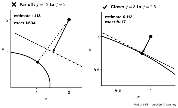
Wrong beside right. Far from a curved level set the first-order distance is badly off; close to it the estimate is good.
“\({\abs{f - c}/\norm{\nabla f}}\) is the distance to the level set.”
Only to first order. From \({(2, 2)}\) on the bowl, where \({f = 12}\), to the contour \({f = 2}\) the estimate is \({10/\sqrt{80} \approx 1.118}\), but the true distance is about 1.634. From \({(1, 1)}\) to \({f = 2.5}\) it is 0.112 against 0.117. Use it near the level set, or for linear functions, where it is exact. At a point where \({\nabla f = \vect{0}}\) it is not defined at all.
“The normal to a surface points at its centre.”
Only on a sphere. On the ellipsoid \({x^2 + 2y^2 + 3z^2 = 6}\) at \({(1, 1, 1)}\) the normal is \({(1, 2, 3)}\), \({22.2^\circ}\) away from the radius \({(1, 1, 1)}\). Use the gradient, never the radius.
“Changing each feature by a tiny amount barely changes the input.”
A change of \(\epsilon\) in each of \(n\) coordinates has ordinary length \({\epsilon\sqrt{n}}\), and it can move a linear score by \({\epsilon\norm{\vect{w}}_1}\), which grows like \(n\). For 784 pixels at \({\epsilon = 0.01}\) the step is 0.28 long and the score can move by several units. That is why imperceptible perturbations can fool image classifiers.
Check yourself
Recall
1. What is the tangent plane to the level surface of \(f\) through \(\vect{a}\)?
Show answer
\({\nabla f(\vect{a})\T(\vect{x} - \vect{a})} = {0}\): the plane through \(\vect{a}\) at right angles to the gradient.
2. What is the first-order distance from \(\vect{x}\) to the level set \({f = c}\)?
When \(f\) is linear (affine), \({\vect{w}\T\vect{x} + b}\): the level sets are hyperplanes and the linear model is \(f\) itself.
4. What is the smallest L2 step that changes the score \({\vect{w}\T\vect{x} + b}\) by \(\Delta\)?
Show answer
\({\Delta\,\vect{w}/\norm{\vect{w}}^2}\), of length \({\abs{\Delta}/\norm{\vect{w}}}\).
5. What perturbation does the fast gradient sign method add to an input?
Show answer
\({\epsilon\operatorname{sign}(\nabla_{\vect{x}} J)}\): the steepest-ascent step of the loss in the max-norm, every input moving by \(\epsilon\).
Exercises
1.★ Find the tangent plane to \({x^2 + y^2 + z^2 = 14}\) at \({(1, 2, 3)}\) and its distance from the origin.
Show solution
\({\nabla f = (2, 4, 6)}\), so \({2(x - 1) + 4(y - 2) + 6(z - 3) = 0}\), that is \({x + 2y + 3z = 14}\). Its distance from the origin is \({14/\sqrt{1 + 4 + 9}} = {14/\sqrt{14}} = {\sqrt{14}}\), the radius of the sphere.
2.★★ Find the distance from \({(3, 2)}\) to the line \({3x + 4y = 5}\), the nearest point on it, and the smallest max-norm step that reaches it.
Show solution
The score \({3x + 4y - 5}\) is \({9 + 8 - 5 = 12}\) at \({(3, 2)}\), so the distance is \({12/5 = 2.4}\). The nearest point is \({(3, 2) - \tfrac{12}{25}(3, 4)} = {(1.56, 0.08)}\); check: \({4.68 + 0.32 = 5}\). In the max-norm the score falls by at most \({7\epsilon}\), so the smallest step has \({\epsilon = 12/7 \approx 1.714}\), along \({-(1, 1)}\).
3.★★★ For logistic regression \({p = \sigma(\vect{w}\T\vect{x} + b)}\) with log loss \({J = -y\ln p - (1 - y)\ln(1 - p)}\), show that \({\nabla_{\vect{x}} J = (p - y)\,\vect{w}}\). Then, with \({\vect{w} = (3, 4)}\), \({b = -5}\), \({\vect{x} = (2, 1)}\) and \({y = 1}\), find the smallest \(\epsilon\) for which the sign attack changes the predicted class.
Each \(x_i\) enters \(z\) with coefficient \(w_i\), so \({\pd{J}{x_i} = (p - y)\,w_i}\) and \({\nabla_{\vect{x}} J = (p - y)\,\vect{w}}\). Here \({p - y < 0}\), so the attack adds \({-\epsilon(1, 1)}\) and lowers the score by \({7\epsilon}\) from 5. The class changes when the score drops below 0, so \({\epsilon > 5/7 \approx 0.714}\) (at exactly \({5/7}\) the point sits on the boundary).
Summary card
The gradient is a normal: it gives the tangent plane, and dividing by its length gives the distance to a level set.
Sources. Each was opened and checked against this lesson on 15 November 2026.
Denis Auroux, MIT OpenCourseWare 18.02SC Multivariable Calculus, Session 36: Proof: the reading proves that at a point of a level surface \({f(x, y, z) = c}\) the gradient is perpendicular to the tangent of every curve on the surface through the point.
Gilbert Strang and Edwin Herman, Calculus Volume 3 (OpenStax), Section 4.6: Theorem 4.14 (the gradient is normal to the level curve), the gradient in three variables (Equation 4.40), and exercises on tangent planes and normal lines to level surfaces.
Ian Goodfellow, Jonathon Shlens and Christian Szegedy, Explaining and Harnessing Adversarial Examples, ICLR 2015: Section 3 (under a max-norm limit the perturbation \({\epsilon\operatorname{sign}(\vect{w})}\) changes \({\vect{w}\T\vect{x}}\) most, by an amount that grows with the dimension), Section 4 (the fast gradient sign method, \({\epsilon\operatorname{sign}(\nabla_{\vect{x}} J)}\)) and Section 5 (for logistic regression the method is exact, and \({\vect{w}\T\operatorname{sign}(\vect{w})} = {\norm{\vect{w}}_1}\)).
SciPy 1.18 reference, scipy.optimize.minimize: constraints for SLSQP are given as dictionaries with a type of 'eq' or 'ineq' and a function fun; an equality constraint asks that function to be zero.
Next. M05.4 (Jacobians and the multivariable chain rule) moves from one output to many: the gradient becomes a row of the Jacobian, and the chain rule proves the right angle of lesson 2 a second way. Margins of classifiers return in ML02.7.