Steepest descent compares steps of length 1, so the answer depends on the ruler. In L2 it is minus the gradient, in the max-norm minus its sign, in L1 a single coordinate, and in a quadratic norm the preconditioned step minus A inverse times the gradient.
M05.3.3L2 Intermediate25 minIn review (what this means)
The maths and code on this page are checked by automated tests on every change, but an independent reader has not signed it off yet. Spot a mistake or a confusing step? Tell us.
Define the normalised steepest-descent direction of a norm as the unit step that most decreases the linear model.
Derive the steepest-descent direction and its slope in the L2 norm, the max-norm and the L1 norm.
Derive minus A inverse times the gradient as the steepest direction in the norm square root of d transpose A d, by a change of variable.
Connect sign-based optimisers, coordinate descent and preconditioning to the choice of norm.
Find each steepest direction by brute force over the unit ball and check it against its formula.
The question
Lesson 2 proved that minus the gradient is the steepest way down. But “steepest” compares steps of the same size, and size was measured with the ordinary ruler. What if every weight may move by at most 0.01, or only one weight may move at a time, or some weights are far more sensitive than others? Does the best direction stay the same?
From the last lesson
1. In which direction does \(f\) fall fastest, and at what slope?
Show answer
Along \({-\nabla f/\norm{\nabla f}}\), at slope \({-\norm{\nabla f}}\).
2. What is the steepest slope of the running bowl at \({(1, 1)}\)?
Show answer
\({\norm{(2, 4)} = \sqrt{20} \approx 4.472}\).
Intuition
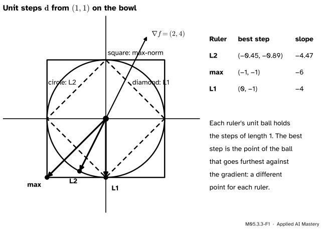
To compare steps fairly we fix their size. All steps of size 1 make up the unit ball of a ruler, and the best step is the point of that ball that goes furthest against the gradient. Change the ruler and the ball changes shape: a circle for the ordinary length, a square when the largest single move counts, a diamond when the moves add up. The furthest point moves with it.
M05.3.3-F1
One gradient, three rulers, three best steps. Each arrow ends at the point of its unit ball that goes furthest against \({\nabla f = (2, 4)}\).
So “steepest” is not a property of the function alone. It belongs to the function and the ruler together, and machine learning uses several rulers on purpose.
Build it up
Step 1. Why a ruler is needed. For a small step \(\vect{d}\) the change in \(f\) is about \({\nabla f\T\vect{d}}\) (lesson 1). Double \(\vect{d}\) and this doubles, so without a limit on the size of the step there is no best step at all. We ask for the most negative \({\nabla f\T\vect{d}}\) among steps with \({\norm{\vect{d}} \le 1}\), for a chosen norm (M02.3.2).
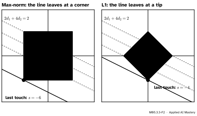
Step 2. Slide a line across the ball. The steps with \({\nabla f\T\vect{d} = s}\) form a line at right angles to the gradient, and lowering \(s\) slides the line across the ball. The best step is the last point the line touches. For \({\nabla f = (2, 4)}\) the line \({2d_1 + 4d_2 = s}\) last touches the square at the corner \({(-1, -1)}\), where \({s = -6}\), and the diamond at the tip \({(0, -1)}\), where \({s = -4}\).
M05.3.3-F2
Lines of equal \({\nabla f\T\vect{d}}\) slide down across the ball. A square is left last at a corner, a diamond at a tip.
Step 3. Corners and tips in \(n\) dimensions. The max-norm ball in \(\R^n\) is a cube whose corners are the \({2^n}\) vectors of \(\pm 1\) entries; the L1 ball has \({2n}\) tips, \({\pm\vect{e}_i}\). A line, now a flat hyperplane, leaves a cube at a corner and an L1 ball at a tip, so the answers of Step 2 carry over.
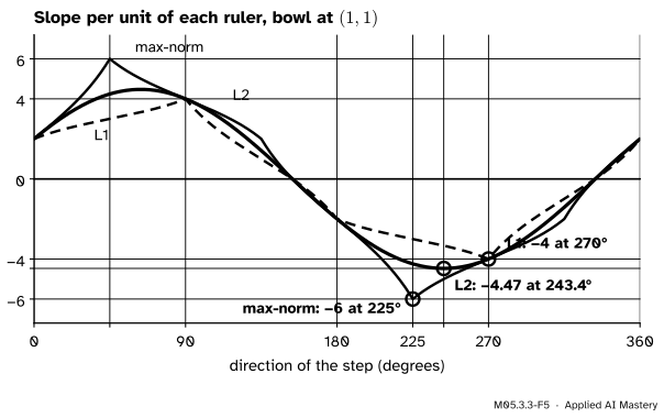
Step 4. Slope per unit of each ruler. Measure the slope as the change of the linear model per unit of the chosen ruler, \({\nabla f\T\vect{v} / \norm{\vect{v}}}\), and draw it against the direction of \(\vect{v}\). Each ruler gives its own curve, and each curve bottoms out at its own direction.
M05.3.3-F5
The bowl at \({(1, 1)}\): the slope per unit of each ruler. The lowest points sit at \({243.4^\circ}\) (L2), \({225^\circ}\) (max-norm) and \({270^\circ}\) (L1).
The formal statement
NoteDefinition: steepest descent for a norm
Given a norm \({\norm{\cdot}}\) on \(\R^n\) and \({\vect{g}} = {\nabla f(\vect{a}) \neq \vect{0}}\), a normalised steepest-descent direction is a step \(\vect{d}\) with \({\norm{\vect{d}} \le 1}\) that makes \({\vect{g}\T\vect{d}}\) as small as possible. The smallest value is the steepest slope per unit of that norm. Steepest ascent is minus the same step.
NoteResults: four rulers
Norm
Best step
Slope
L2
\({-\vect{g}/\norm{\vect{g}}}\)
\({-\norm{\vect{g}}}\)
max
\({-\operatorname{sign}(\vect{g})}\)
\({-\norm{\vect{g}}_1}\)
L1
\({-\operatorname{sign}(g_k)\vect{e}_k}\)
\({-\norm{\vect{g}}_\infty}\)
\(\mat{A}\)
\({\propto -\mat{A}^{-1}\vect{g}}\)
\({-\norm{\vect{g}}_{\mat{A}^{-1}}}\)
Here \(k\) is an index with the largest \({\abs{g_k}}\); the \(\mat{A}\)-norm is \({\norm{\vect{d}}_{\mat{A}} = \sqrt{\vect{d}\T\mat{A}\vect{d}}}\) for a symmetric positive definite \(\mat{A}\), so \({\norm{\vect{g}}_{\mat{A}^{-1}} = \sqrt{\vect{g}\T\mat{A}^{-1}\vect{g}}}\).
L2 is lesson 2.
Max-norm. Here \({\norm{\vect{d}}_\infty} = {\max_i \abs{d_i}} \le {1}\), so every \({\abs{d_i} \le 1}\). Each term of the dot product is then at least \({-\abs{g_i}}\):
Equality needs \({d_i = -\operatorname{sign}(g_i)}\) wherever \({g_i \neq 0}\): every coordinate moves by the full amount, against the sign of its partial derivative.
L1. Here \({\sum_i \abs{d_i} \le 1}\), and every \({\abs{g_i}}\) is at most \({\abs{g_k} = \norm{\vect{g}}_\infty}\):
The step \({-\operatorname{sign}(g_k)\,\vect{e}_k}\) reaches it: only the coordinate with the largest partial derivative moves. When several tie, any mix of them along the edge between their tips does as well.
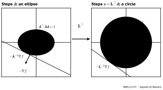
A quadratic norm. Let \({\norm{\vect{d}}_{\mat{A}}} = {\sqrt{\vect{d}\T\mat{A}\vect{d}}}\). Its unit ball is an ellipse, and a change of variable turns it into a circle. Factor \({\mat{A} = \mat{L}\mat{L}\T}\) by Cholesky (M03.4.3), so that \({\vect{d}\T\mat{A}\vect{d}} = {\norm{\mat{L}\T\vect{d}}^2}\), and put \({\vect{e} = \mat{L}\T\vect{d}}\), that is \({\vect{d} = \mat{L}^{-\top}\vect{e}}\). Then
with \({\norm{\vect{e}} \le 1}\). This is the L2 problem for the vector \({\mat{L}^{-1}\vect{g}}\), so \({\vect{e}} = {-\mat{L}^{-1}\vect{g}/\norm{\mat{L}^{-1}\vect{g}}}\). Back in \(\vect{d}\):
because \({\mat{A}^{-1}} = {(\mat{L}\mat{L}\T)^{-1}} = {\mat{L}^{-\top}\mat{L}^{-1}}\) and \({\norm{\mat{L}^{-1}\vect{g}}^2} = {\vect{g}\T\mat{L}^{-\top}\mat{L}^{-1}\vect{g}} = {\vect{g}\T\mat{A}^{-1}\vect{g}}\). The slope is \({\vect{g}\T\vect{d}} = {-\sqrt{\vect{g}\T\mat{A}^{-1}\vect{g}}}\).
M05.3.3-F3
The change of variable \({\vect{e} = \mat{L}\T\vect{d}}\) turns the ellipse into a circle, where the answer is minus the (new) gradient. Mapped back, it is \({-\mat{A}^{-1}\nabla f}\), not \({-\nabla f}\).
Go deeper: dual norms: the pattern in the slope column
The slope column pairs each ruler with another norm: L2 with L2, the max-norm with L1, L1 with the max-norm, and \({\norm{\cdot}_{\mat{A}}}\) with \({\norm{\cdot}_{\mat{A}^{-1}}}\). The partner is the dual norm, \({\norm{\vect{g}}_*} = {\max\{\vect{g}\T\vect{d} : \norm{\vect{d}} \le 1\}}\), so by definition the steepest slope is \({-\norm{\vect{g}}_*}\). Boyd and Vandenberghe build steepest descent on this pairing, scaling the normalised step by \({\norm{\nabla f}_*}\) (their Equation 9.24); for a quadratic norm the scaled step is exactly \({-\mat{A}^{-1}\nabla f}\) (Equation 9.25).
Worked example
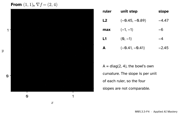
The bowl at \({(1, 1)}\), \({\vect{g} = (2, 4)}\), in all four rulers.
L1: the larger entry is \({g_2 = 4}\), so the step is \({(0, -1)}\), slope \(-4\).
\({\mat{A} = \operatorname{diag}(2, 4)}\), the bowl’s own curvature: \({\mat{A}^{-1}\vect{g}} = {(2/2,\, 4/4)} = {(1, 1)}\) and \({\vect{g}\T\mat{A}^{-1}\vect{g}} = {2 + 4} = {6}\). The step is \({-(1, 1)/\sqrt{6}} \approx {(-0.408, -0.408)}\), slope \({-\sqrt{6} \approx -2.449}\). Check the size: \({(2 \cdot 1 + 4 \cdot 1)/6 = 1}\).
The last direction points from \({(1, 1)}\) straight at the minimum \({(0, 0)}\). That is no luck: the bowl is \({\tfrac12\vect{x}\T\mat{A}\vect{x}}\) with this \(\mat{A}\), so \({\nabla f = \mat{A}\vect{x}}\) and \({-\mat{A}^{-1}\nabla f = -\vect{x}}\), the arrow home from any point. That is the Newton step, met again in M05.5.4 and M08.5. At \({(1, 1)}\) it happens to share its direction with the max-norm step; at \({(2, 1)}\), where \({\vect{g} = (4, 4)}\), the max-norm still says \({(-1, -1)}\) but \({-\mat{A}^{-1}\vect{g} = -(2, 1)}\).
M05.3.3-F4
The worked example as a trace. The quadratic-norm step with the bowl’s own curvature aims exactly at the minimum.
Where machine learning uses each ruler. Moving every weight by the same amount against the sign of its partial derivative is the max-norm step: signSGD (Bernstein and coauthors, 2018) updates with the sign of a mini-batch gradient, and the fast gradient sign attack of lesson 4 moves every pixel by the same small amount. Moving one coordinate at a time is the L1 step, the idea of coordinate descent. Rescaling the gradient by \({\mat{A}^{-1}}\) is preconditioning: with the Hessian as \(\mat{A}\) it is Newton’s method (M08.5), and adaptive optimisers that scale each weight separately (M08.4) choose a diagonal \(\mat{A}\). With the Fisher information matrix of a probabilistic model as \(\mat{A}\) it is the natural gradient: steepest descent when the size of a small step is measured by how much the model’s predicted distribution changes (Martens, 2020), used for policies in RL04.6.
Code
Brute force in the plane: put many directions on each unit ball, keep the one with the smallest \({\nabla f\T\vect{d}}\), and compare it with the formula.
import numpy as npg = np.array([2.0, 4.0])A = np.diag([2.0, 4.0])theta = np.linspace(0, 2* np.pi, 3600, endpoint=False)v = np.stack([np.cos(theta), np.sin(theta)], axis=1) # directions, one per rowrulers = {"L2": np.linalg.norm(v, axis=1),"max": np.max(np.abs(v), axis=1),"L1": np.sum(np.abs(v), axis=1),"A": np.sqrt(np.einsum("ij,jk,ik->i", v, A, v))}formula = {"L2": -g / np.linalg.norm(g), "max": -np.sign(g), "L1": np.array([0.0, -1.0]),"A": -np.linalg.solve(A, g) / np.sqrt(g @ np.linalg.solve(A, g))}found = {}for name, size in rulers.items(): d = v / size[:, None] # every direction scaled to size 1 best = d[np.argmin(d @ g)] found[name] = bestprint(f"{name:4s} brute force {np.round(best, 3)} formula {np.round(formula[name], 3)}"f" slope {best @ g:.3f}")
L2   brute force [-0.448 -0.894]  formula [-0.447 -0.894]  slope -4.472
max  brute force [-1. -1.]  formula [-1. -1.]  slope -6.000
L1   brute force [-0. -1.]  formula [ 0. -1.]  slope -4.000
A    brute force [-0.408 -0.408]  formula [-0.408 -0.408]  slope -2.449
In more dimensions the corners can be listed exactly. For a random gradient in \(\R^8\), all \({2^8 = 256}\) corners of the cube and all 16 tips of the L1 ball are tried; the quadratic norm is checked against a hundred thousand random points of its ellipsoid.
from itertools import productrng = np.random.default_rng(3)n =8g8 = rng.normal(size=n)corners = np.array(list(product([-1.0, 1.0], repeat=n)))tips = np.vstack([np.eye(n), -np.eye(n)])print("max-norm: best corner", (corners @ g8).min().round(4), " -||g||_1 =", (-np.abs(g8).sum()).round(4))print("L1: best tip ", (tips @ g8).min().round(4), " -||g||_inf =", (-np.abs(g8).max()).round(4))M = rng.normal(size=(n, n))A8 = M @ M.T + n * np.eye(n) # symmetric positive definiteL8 = np.linalg.cholesky(A8)e = rng.normal(size=(100_000, n))e /= np.linalg.norm(e, axis=1, keepdims=True)d = np.linalg.solve(L8.T, e.T).T # d = L^{-T} e has d^T A d = 1exact =-np.sqrt(g8 @ np.linalg.solve(A8, g8))print("A-norm: best sample", (d @ g8).min().round(4), " formula", exact.round(4))
max-norm: best corner -8.5026   -||g||_1 = -8.5026
L1:       best tip    -2.5557   -||g||_inf = -2.5557
A-norm:   best sample -0.9297   formula -0.9546
The corners and tips match the formulas exactly. The random samples of the ellipsoid come close to the formula from above but never pass it, as a bound must.
Explore
M05.3-X1
Direction dial
Drag the orange point on the contour map, or set it with the sliders, and turn the direction. The side panel plots the slope against the angle: a cosine with its peak along the gradient and zeros along the contour line. Switch the ruler to L1 or the max-norm to see its unit ball and the steepest-ascent step it picks (minus the descent step of this lesson), beside the gradient.
Pitfalls
M05.3.3-F6
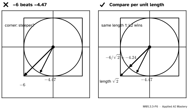
Wrong beside right. The corner step is \({\sqrt{2}}\) long, so its \(-6\) is not a steeper slope. Shrunk to length 1, the same direction falls at only \({-6/\sqrt{2} \approx -4.24}\).
“The max-norm direction is steeper: \(-6\) beats \(-4.47\).”
Each slope is per unit of its own ruler. The corner \({(-1, -1)}\) has max-norm 1 but ordinary length \({\sqrt{2}}\), so per unit of ordinary length it falls at \({-6/\sqrt{2} \approx -4.24}\), less steep than \(-4.47\), as lesson 2 promised. In \({\R^n}\) a corner is \({\sqrt{n}}\) long, which is why a sign step can change a function a lot while each coordinate moves only a little.
“The sign of the gradient is the gradient, rescaled.”
It is not parallel to it. \({\operatorname{sign}(2, 4) = (1, 1)}\) points at \({45^\circ}\) while \({(2, 4)}\) points at \({63.4^\circ}\), \({18.4^\circ}\) apart. The sign throws away the sizes of the partial derivatives and keeps only their directions, which is exactly what a max-norm budget asks for.
“The steepest direction belongs to the function.”
It belongs to the function and the ruler. Measure one input in different units, centimetres instead of metres, and the ordinary ruler on the new numbers is a different ruler on the old ones: a quadratic norm with a diagonal \(\mat{A}\). So rescaling features changes which way gradient descent goes, the effect that M03.8.4 used to cure a zigzag.
Check yourself
Recall
1. What is the normalised steepest-descent direction of a norm?
Show answer
A step \(\vect{d}\) with \({\norm{\vect{d}} \le 1}\) that makes \({\nabla f\T\vect{d}}\) as small as possible.
2. What is it in the max-norm, and what is the slope?
Show answer
\({-\operatorname{sign}(\nabla f)}\), every coordinate moving by 1; the slope is \({-\norm{\nabla f}_1}\), minus the sum of the absolute partial derivatives.
3. What is it in the L1 norm?
Show answer
Move only the coordinate \(k\) with the largest \({\abs{\partial f/\partial x_k}}\), by 1 against its sign; the slope is \({-\norm{\nabla f}_\infty}\).
4. In the norm \({\sqrt{\vect{d}\T\mat{A}\vect{d}}}\), which way is steepest descent?
Show answer
Along \({-\mat{A}^{-1}\nabla f}\), scaled to size 1 by dividing by \({\sqrt{\nabla f\T\mat{A}^{-1}\nabla f}}\).
5. Match each ruler with an idea from training: sign methods, coordinate descent, preconditioning.
Show answer
Max-norm with sign methods (signSGD, the fast gradient sign attack), L1 with coordinate descent, and the quadratic norm with preconditioning (Newton’s method, per-weight scaling).
Exercises
1.★ For \({\vect{g} = (3, -1, 2)}\), give the steepest-descent step and slope in the L2 norm, the max-norm and the L1 norm.
Show solution
L2: \({-(3, -1, 2)/\sqrt{14}}\), slope \({-\sqrt{14} \approx -3.742}\). Max-norm: \({-\operatorname{sign}(\vect{g})} = {(-1, 1, -1)}\), slope \({-(3 + 1 + 2) = -6}\). L1: the largest entry is \({g_1 = 3}\), so the step is \({(-1, 0, 0)}\), slope \(-3\).
2.★★ On the bowl at \({(2, 1)}\) with \({\mat{A} = \operatorname{diag}(2, 4)}\), find the steepest-descent step in the \(\mat{A}\)-norm and its slope, and the steps of the max-norm and L1.
Show solution
\({\vect{g} = (4, 4)}\), \({\mat{A}^{-1}\vect{g} = (2, 1)}\) and \({\vect{g}\T\mat{A}^{-1}\vect{g}} = {8 + 4} = {12}\). The step is \({-(2, 1)/\sqrt{12}} \approx {(-0.577, -0.289)}\), slope \({-\sqrt{12} \approx -3.464}\), and \({(2, 1) - (2, 1) = (0, 0)}\): it aims at the minimum. Max-norm: \({(-1, -1)}\), slope \(-8\). L1: the two entries tie at 4, so \({(-1, 0)}\), \({(0, -1)}\) and every step on the edge between them give slope \(-4\).
3.★★★ Let \({f(\vect{x})} = {\tfrac12\vect{x}\T\mat{A}\vect{x}}\) with \(\mat{A}\) symmetric positive definite. Show that the unscaled step \({-\mat{A}^{-1}\nabla f}\) lands on the minimum from every point, and that for a diagonal \({\mat{A}} = {\operatorname{diag}(a_1, \dots, a_n)}\) it divides each partial derivative by its own \(a_i\).
Show solution
The gradient of \({\tfrac12\vect{x}\T\mat{A}\vect{x}}\) is \({\mat{A}\vect{x}}\) for symmetric \(\mat{A}\) (M05.7.1 derives it; here it can be checked entry by entry). So \({-\mat{A}^{-1}\nabla f} = {-\mat{A}^{-1}\mat{A}\vect{x}} = {-\vect{x}}\), and \({\vect{x} + (-\vect{x}) = \vect{0}}\), the minimum, since \({f \ge 0 = f(\vect{0})}\) for a positive definite \(\mat{A}\). For a diagonal \(\mat{A}\) the inverse is \({\operatorname{diag}(1/a_1, \dots, 1/a_n)}\), so entry \(i\) of \({-\mat{A}^{-1}\nabla f}\) is \({-(\partial f/\partial x_i)/a_i}\): each coordinate gets its own step size.
Summary card
Steepest descent is the point of the unit ball that goes furthest against the gradient, so it depends on the ruler.
L1: one coordinate, the largest partial derivative; slope \({-\norm{\nabla f}_\infty}\).
\({\sqrt{\vect{d}\T\mat{A}\vect{d}}}\): along \({-\mat{A}^{-1}\nabla f}\), slope \({-\sqrt{\nabla f\T\mat{A}^{-1}\nabla f}}\).
Bowl at \({(1, 1)}\): \(-4.47\), \(-6\), \(-4\), \(-2.45\).
Sources and next steps
Sources. Each was opened and checked against this lesson on 15 November 2026.
Stephen Boyd and Lieven Vandenberghe, Convex Optimization, Cambridge University Press, 2004 (free PDF from the authors), Section 9.4: the normalised steepest-descent direction as the minimiser of \({\nabla f\T\vect{v}}\) over unit steps of any norm (Equation 9.23), the step scaled by the dual norm (Equation 9.24), the Euclidean case (gradient descent) and the quadratic norm, whose step is \({-\mat{P}^{-1}\nabla f}\) (Equation 9.25) and equals gradient descent after the change of coordinates \({\mat{P}^{1/2}\vect{x}}\) (Section 9.4.1), and the L1 norm, whose step moves one coordinate and gives coordinate descent (Section 9.4.2).
Jeremy Bernstein, Yu-Xiang Wang, Kamyar Azizzadenesheli and Anima Anandkumar, signSGD: Compressed Optimisation for Non-Convex Problems, 2018: the abstract describes transmitting only the sign of each mini-batch gradient, and reports that signSGD with momentum matched Adam’s accuracy and speed on deep ImageNet models.
Ian Goodfellow, Jonathon Shlens and Christian Szegedy, Explaining and Harnessing Adversarial Examples, ICLR 2015, Section 3: under a max-norm limit on a perturbation \(\vect{\eta}\), the change \({\vect{w}\T\vect{\eta}}\) is largest at \({\vect{\eta}} = {\epsilon\operatorname{sign}(\vect{w})}\).
James Martens, New Insights and Perspectives on the Natural Gradient Method, Journal of Machine Learning Research 21, 2020 (opened and checked on 15 November 2026), Section 6: minus \({\mat{A}^{-1}\nabla f}\) is the limiting steepest-descent direction for the norm \({\sqrt{\vect{d}\T\mat{A}\vect{d}}}\), and with the Fisher matrix in place of \(\mat{A}\) this makes the negative natural gradient the steepest descent direction in the space of distributions.