The gradient was built from slopes along the axes, yet it predicts the change of a function for a small step in any direction. That prediction is the tangent plane, and a function is differentiable exactly when its error shrinks faster than the step.
M05.2.2L2 Intermediate25 minIn review (what this means)
The maths and code on this page are checked by automated tests on every change, but an independent reader has not signed it off yet. Spot a mistake or a confusing step? Tell us.
Write the linear model f(a + h) ≈ f(a) + ∇f(a)ᵀh and compute its remainder for a given step.
State the definition of differentiability, that the remainder divided by the step length tends to 0, and show that the vector in it must be the gradient.
Write the tangent plane of a function of two variables at a point, with its partial derivatives in full.
Explain with xy/(x² + y²) why partial derivatives can exist where there is no tangent plane, and state the condition that guarantees one.
Tabulate the remainder over the step length for shrinking steps and read off whether it tends to 0.
The question
Gradient descent never moves one weight at a time. Every step changes all of them at once, in a direction that is almost never along an axis. Yet the gradient is built only from slopes along the axes. Can \(n\) axis slopes really predict what happens for a step in any direction? When they can, how good is the prediction, and is there a function where they fail?
From the last lesson
1. What is the gradient of \({\vect{w}\T\vect{x}}\) with respect to \(\vect{x}\)?
Show answer
\(\vect{w}\), the same at every point.
2. Where does the norm \({\norm{\vect{x}}}\) have no gradient, and why?
Show answer
At the origin. Along every axis it is \({\abs{t}}\), which has a corner at 0, so no partial derivative exists there.
Intuition
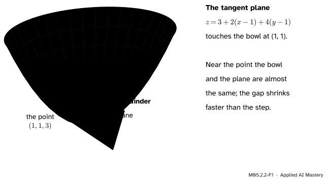
Zoom in on a smooth surface at a point and it looks flatter and flatter, until it is indistinguishable from a plane. That plane is the tangent plane: the two-input version of the tangent line of M04.2.2. Its tilt in each axis direction is the partial derivative, so the gradient fixes it completely.
Step away from the point by a small step \(\vect{h}\). The plane predicts a height; the surface has another. The gap between them is the remainder. A tangent plane deserves the name when that gap shrinks faster than the step.
M05.2.2-F1
The tangent plane of the running bowl at \({(1, 1)}\). For a step \(\vect{h}\) the plane predicts one height and the bowl has another; the gap between them, the remainder, is drawn in purple.
A curve that fits the plane at a point only to first order still pulls away from it. What matters is the rate: halve the step and, for the bowl, the gap falls to a quarter.
Build it up
Step 1. The linear model. M04.10.3 split a small step into moves along each axis and added the changes. With \(n\) inputs the same idea predicts
The prediction \({\cmodel{\nabla f(\vect{a})\T\vect{h}}}\) is a dot product: the gradient’s entries weighted by how far each input moves. This is the linear model of \(f\) at \(\vect{a}\).
Step 2. Name the error. The remainder is whatever the linear model misses:
The first three terms are \({f(1, 1) = 3}\) and \({\nabla f\T\vect{h} = 2h_1 + 4h_2}\), so the remainder is \({r(\vect{h}) = h_1^2 + 2h_2^2}\).
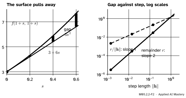
Step 3. Compare the error with the step. Shrink the step along the diagonal, \({\vect{h} = (s, s)}\). Then \({r = 3s^2}\) and \({\norm{\vect{h}} = \sqrt{2}\,s}\), so
As \(s\) goes to 0, so does the ratio. The remainder is not just small; it is small compared with the step.
M05.2.2-F2
Left: along the diagonal from \({(1, 1)}\) the bowl rises as \({3 + 6s + 3s^2}\) and the linear model as \({3 + 6s}\). Right: on log scales the remainder falls with slope 2 and the remainder per unit of step with slope 1: both tend to 0.
Any direction behaves the same way. Since \({h_1^2 + 2h_2^2 \le 2h_1^2 + 2h_2^2 = 2\norm{\vect{h}}^2}\), we get \({0 \le r(\vect{h})/\norm{\vect{h}} \le 2\norm{\vect{h}}}\), which tends to 0 however the step shrinks.
The formal statement
NoteDefinition: differentiable
\({f : \R^n \to \R}\) is differentiable at \(\vect{a}\) if there is a vector \(\vect{g}\) such that, for all small steps \(\vect{h}\),
The vector must be the gradient. Take the step along axis \(i\), \({\vect{h} = t\,\vect{e}_i}\). Then \({\vect{g}\T\vect{h} = t\,g_i}\) and \({\norm{\vect{h}} = \abs{t}}\), and dividing the definition by \(t\) gives
The last term has the size of \({r/\norm{\vect{h}}}\), so it tends to 0. The left side therefore tends to \(g_i\), which says that the partial derivative exists and equals \(g_i\). So \({\vect{g} = \nabla f(\vect{a})}\): if any linear model has a remainder that vanishes faster than the step, it is the one built from the gradient.
The tangent plane. In two variables, with \({\vect{a} = (a_1, a_2)}\) and the step \({\vect{h} = (x - a_1, y - a_2)}\), the graph of the linear model is the plane
Differentiable means continuous. Letting \({\vect{h} \to \vect{0}}\) in the definition, \({\vect{g}\T\vect{h} \to 0}\) and \({r(\vect{h}) = \norm{\vect{h}} \cdot (r/\norm{\vect{h}}) \to 0}\), so \({f(\vect{a} + \vect{h}) \to f(\vect{a})}\).
Partial derivatives are not enough. Let \({k(x, y) = xy/(x^2 + y^2)}\), with \({k(0, 0) = 0}\), the function of M05.1.4. On both axes \(k\) is 0, so both partial derivatives at the origin are 0. If \(k\) were differentiable there, the vector would be \({\vect{g} = (0, 0)}\) and the remainder would be \({r(\vect{h}) = k(\vect{h})}\). Along the diagonal, \({\vect{h} = (t, t)}\):
which grows without bound as \(t\) shrinks. So \(k\) has two partial derivatives at the origin and no tangent plane. (It is not even continuous there, which M05.1.4 showed.)
NoteResult: a sufficient condition
If all the partial derivatives of \(f\) exist near \(\vect{a}\) and are continuous at \(\vect{a}\), then \(f\) is differentiable at \(\vect{a}\).
Every polynomial, the sigmoid, the logarithm on its domain and every loss built from them pass this test wherever they are defined, which is why training can trust the linear model almost everywhere. The ReLU and the norm fail it at their corners.
M05.2.2-F5
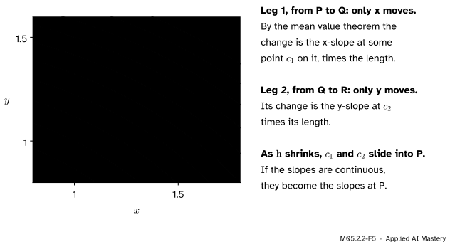
Why continuous partial derivatives are enough, in two variables. Each leg of the path moves one input, so each change is a one-variable slope times a length.
Go deeper: the proof of the sufficient condition, in two variables
On the first leg only \(x\) moves, so by the mean value theorem (M04.4) there is a point \(c_1\) between \(a_1\) and \({a_1 + h_1}\) with \({f(Q) - f(P) = f_x(c_1, a_2)\,h_1}\), where \(f_x\) is \({\pd{f}{x}}\). In the same way there is \(c_2\) between \(a_2\) and \({a_2 + h_2}\) with \({f(R) - f(Q) = f_y(a_1 + h_1, c_2)\,h_2}\). Subtract the linear model:
Since \({\abs{h_1}, \abs{h_2} \le \norm{\vect{h}}}\), dividing by \({\norm{\vect{h}}}\) leaves at most the sum of the two bracketed differences in size. As \({\vect{h} \to \vect{0}}\) the points \({(c_1, a_2)}\) and \({(a_1 + h_1, c_2)}\) tend to \(P\), and continuity of \(f_x\) and \(f_y\) at \(P\) sends both brackets to 0. So \({r(\vect{h})/\norm{\vect{h}} \to 0}\). With \(n\) inputs the path has \(n\) legs and the argument is the same.
Worked example
The bowl at \({(1, 1)}\). Here \({f = 3}\), \({\pd{f}{x} = 2}\) and \({\pd{f}{y} = 4}\), so the tangent plane is
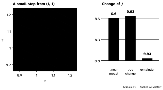
Step by \({\vect{h} = (0.1, 0.1)}\). The plane predicts \({2.2 + 4.4 - 3 = 3.6}\), a rise of \({\nabla f\T\vect{h} = 0.2 + 0.4 = 0.6}\). The bowl gives \({f(1.1, 1.1) = 1.21 + 2.42 = 3.63}\), a rise of 0.63. The remainder is \({0.03 = 0.1^2 + 2 \times 0.1^2}\), as Step 2 predicted.
M05.2.2-F3
The worked example. The step \(\vect{h}\) crosses from the contour line \({f = 3}\) to \({f = 3.63}\). The linear model \({\nabla f\T\vect{h}}\) predicts a rise of 0.6; the true rise is 0.63; the remainder is 0.03.
Shrink the step by ten, twice:
step \({(s, s)}\)
remainder
\({r/\norm{\vect{h}}}\)
\({s = 0.1}\)
0.03
0.2121
\({s = 0.01}\)
0.0003
0.02121
\({s = 0.001}\)
0.000003
0.002121
Each tenfold cut in the step cuts the remainder a hundredfold and the ratio tenfold.
The running loss at the origin.\({L(0, 0) = 18.5}\) and \({\nabla L(0, 0) = (-23.5, -8)}\), so the tangent plane is \({z = 18.5 - 23.5w - 8b}\). For the step \({(0.1, 0.1)}\) it predicts a change of \({-2.35 - 0.8 = -3.15}\). The loss itself is
a change of \(-3.015\). The remainder, \({0.135}\), is exactly the quadratic part \({7.5w^2 + 5wb + b^2}\) of the loss at the step, because a quadratic’s linear model misses only its quadratic terms. M05.5 shows that this part is \({\tfrac12\vect{h}\T\mat{H}\vect{h}}\).
Code
From scratch: the remainder over the step length, for steps that shrink along a fixed direction.
import numpy as npdef ratio_table(f, grad, a, direction, scales=(0.1, 0.01, 0.001)):"""r(h) / ||h|| for h = s * direction, at each scale s.""" a, d = np.asarray(a, float), np.asarray(direction, float) rows = []for s in scales: h = s * d r = f(a + h) - f(a) - grad @ h rows.append((s, r, r / np.linalg.norm(h)))return rowsbowl =lambda v: v[0]**2+2* v[1]**2for s, r, q in ratio_table(bowl, np.array([2.0, 4.0]), [1, 1], [1, 1]):print(f"bowl s = {s:<6} r = {r:.3g} r/|h| = {q:.4g}")def kfun(v): # x y / (x^2 + y^2), and 0 at the origin x, y = vreturn0.0if x ==0and y ==0else x * y / (x**2+ y**2)for s, r, q in ratio_table(kfun, np.zeros(2), [0, 0], [1, 1]):print(f"k at 0 s = {s:<6} r = {r:.3g} r/|h| = {q:.4g}")
bowl  s = 0.1    r = 0.03   r/|h| = 0.2121
bowl  s = 0.01   r = 0.0003   r/|h| = 0.02121
bowl  s = 0.001  r = 3e-06   r/|h| = 0.002121
k at 0  s = 0.1    r = 0.5   r/|h| = 3.536
k at 0  s = 0.01   r = 0.5   r/|h| = 35.36
k at 0  s = 0.001  r = 0.5   r/|h| = 353.6
For the bowl the ratio falls tenfold with each tenfold cut. For \(k\) at the origin the remainder stays at 0.5 and the ratio grows: no tangent plane. Away from the origin \(k\) is a quotient of polynomials with a non-zero denominator, so its partial derivatives are continuous and the sufficient condition applies. At \({(1, 2)}\) they are \({y(y^2 - x^2)/(x^2 + y^2)^2 = 0.24}\) and \({x(x^2 - y^2)/(x^2 + y^2)^2 = -0.12}\) (by the quotient rule, M04.3.3), and the ratio falls again. The same check runs on the running loss.
k at (1, 2)  s = 0.1    r/|h| = -0.0169
k at (1, 2)  s = 0.01   r/|h| = -0.00154
k at (1, 2)  s = 0.001  r/|h| = -0.000153
loss: L(0.1, 0.1) = 15.485  remainder = 0.135
The steps here are moderate on purpose. At steps near \({10^{-8}}\) rounding error would swamp the remainder, a limit that M05.2.4 meets head on.
Explore
M05.2-X1
Linear-model checker
Drag the orange point, or set it with the sliders, and drag the end of the step. The bars compare the linear model’s prediction with the true change, and the graph traces the remainder over the step length as the step shrinks. Shrink it on the bowl and on the loss, then choose \({xy/(x^2 + y^2)}\) and press To the origin.
Pitfalls
M05.2.2-F4
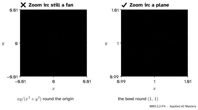
Wrong beside right, both at a zoom of 0.01. \({xy/(x^2 + y^2)}\) looks the same at every scale round the origin, a fan of rays from \(-\tfrac12\) to \(\tfrac12\), so no plane fits it. The bowl, zoomed in as far, has become the contour map of a plane.
“Both partial derivatives exist, so the function has a tangent plane.”
Partial derivatives look only along the axes. \({xy/(x^2 + y^2)}\) is 0 on both axes, so its partial derivatives at the origin are 0, yet along the diagonal it is \(\tfrac12\) at every distance. A tangent plane needs the remainder to vanish faster than the step in every direction at once.
“The linear model is good for any step.”
It is good for small steps. From \({(1, 1)}\) on the bowl, the step \({(1, 1)}\) is predicted to raise \(f\) by \({2 + 4 = 6}\), but \({f(2, 2) = 12}\), a rise of 9. The remainder \({h_1^2 + 2h_2^2 = 3}\) grows like the square of the step. This is why gradient descent with a large learning rate can overshoot.
“Differentiable means the partial derivatives are continuous.”
Continuity of the partial derivatives is enough, but not needed. The function \({\norm{\vect{x}}^2\sin(1/\norm{\vect{x}})}\), with value 0 at the origin, is at most \({\norm{\vect{x}}^2}\) in size, so with \({\vect{g} = \vect{0}}\) the ratio \({r/\norm{\vect{h}}}\) is at most \({\norm{\vect{h}}}\): it is differentiable at 0. Yet its partial derivatives contain a term \({-(x_i/\norm{\vect{x}})\cos(1/\norm{\vect{x}})}\) that keeps swinging as \(\vect{x}\) nears 0.
Check yourself
Recall
1. What is the linear model of \(f\) at \(\vect{a}\) for a step \(\vect{h}\)?
2. What does it mean for \(f\) to be differentiable at \(\vect{a}\)?
Show answer
The remainder \({r(\vect{h}) = f(\vect{a} + \vect{h}) - f(\vect{a}) - \vect{g}\T\vect{h}}\) satisfies \({r(\vect{h})/\norm{\vect{h}} \to 0}\) as \({\vect{h} \to \vect{0}}\) for some vector \(\vect{g}\), which is then the gradient.
3. Write the tangent plane of the bowl \({x^2 + 2y^2}\) at \({(1, 1)}\).
Show answer
\({z = 3 + 2(x - 1) + 4(y - 1)}\), which is \({z = 2x + 4y - 3}\).
4. Why is \({xy/(x^2 + y^2)}\) not differentiable at the origin although both partial derivatives exist?
Show answer
They are 0, so the linear model is 0, but along the diagonal the function is \(\tfrac12\) at every distance: the remainder over the step length grows instead of tending to 0.
5. Which condition guarantees differentiability at a point?
Show answer
All the partial derivatives exist near the point and are continuous at it.
Exercises
1.★ Find the tangent plane of \({f(x, y) = x^2y}\) at \({(1, 2)}\), use it to estimate \({f(1.1, 1.9)}\), and find the remainder.
Show solution
\({f(1, 2) = 2}\), \({\pd{f}{x} = 2xy = 4}\) and \({\pd{f}{y} = x^2 = 1}\) at the point, so the plane is \({z = 2 + 4(x - 1) + (y - 2)}\). At \({(1.1, 1.9)}\) it gives \({2 + 0.4 - 0.1 = 2.3}\). The true value is \({1.21 \times 1.9 = 2.299}\), so the remainder is \({2.299 - 2.3 = -0.001}\).
2.★★ Show from the definition that \({f(x, y) = xy}\) is differentiable at every point \({(a_1, a_2)}\).
Take \({\vect{g} = (a_2, a_1)}\), so \({\vect{g}\T\vect{h} = a_2h_1 + a_1h_2}\) and \({r(\vect{h}) = h_1h_2}\). Since \({0 \le (\abs{h_1} - \abs{h_2})^2}\), we have \({2\abs{h_1h_2} \le h_1^2 + h_2^2 = \norm{\vect{h}}^2}\), so \({\abs{r}/\norm{\vect{h}} \le \norm{\vect{h}}/2}\), which tends to 0. So \(f\) is differentiable with \({\nabla f = (y, x)}\).
3.★★★ Let \({q(x, y) = \sqrt{\abs{xy}}}\). Show that both partial derivatives of \(q\) at the origin are 0, and that \(q\) is not differentiable there.
Show solution
On the \(x\) axis \({q(t, 0) = 0}\) for every \(t\), so the difference quotient is 0 and \({\pd{q}{x}(0, 0) = 0}\); the same holds on the \(y\) axis. If \(q\) were differentiable, the vector would be the gradient \({(0, 0)}\), so \({r(\vect{h}) = q(\vect{h})}\). Along the diagonal \({\vect{h} = (t, t)}\), \({q = \sqrt{t^2} = \abs{t}}\) and \({\norm{\vect{h}} = \sqrt{2}\abs{t}}\), so \({r/\norm{\vect{h}} = 1/\sqrt{2}}\) for every \({t \neq 0}\). It does not tend to 0, so \(q\) is not differentiable at the origin. Unlike \({xy/(x^2 + y^2)}\), \(q\) is continuous there: continuity is not enough either.
Summary card
Differentiable: the tangent plane’s error shrinks faster than the step.
M05.2.2-F1
Plane, step, remainder.
Linear model.\({f(\vect{a} + \vect{h})}\) is \({f(\vect{a}) + \nabla f(\vect{a})\T\vect{h}}\) plus the remainder \({r(\vect{h})}\).
Differentiable.\({r(\vect{h})/\norm{\vect{h}} \to 0}\); the vector is then the gradient.
Tangent plane. The graph of the linear model: \({z = f(\vect{a})}\) plus \({\nabla f(\vect{a})\T(\vect{x} - \vect{a})}\).
Enough. Continuous partial derivatives. Not enough. Partial derivatives alone.
Sources and next steps
Sources. Each was opened and checked against this lesson on 15 November 2026.
Gilbert Strang and Edwin Herman, Calculus Volume 3 (OpenStax), Section 4.4: the tangent plane (Equation 4.24), the definition of differentiability with an error term \(E\) divided by the distance to the point tending to 0 (Equation 4.26), Theorem 4.6 (differentiability implies continuity), Theorem 4.7 (continuous first partials imply differentiability), and \({xy/(x^2 + y^2)}\) as a function whose partial derivatives at the origin exist although it is not differentiable there.
Marc Peter Deisenroth, A. Aldo Faisal and Cheng Soon Ong, Mathematics for Machine Learning, Section 5.8: the gradient as a locally linear approximation of \(f\) around \(\vect{x}_0\) (Equation 5.148).