In the plane a point can be approached along infinitely many paths, and a function can head for different values along different ones. Define limits with a ball of inputs, prove one by a squeeze, disprove one with two paths, and see why the losses of machine learning are continuous.
M05.1.4L2 Intermediate25 minIn review (what this means)
The maths and code on this page are checked by automated tests on every change, but an independent reader has not signed it off yet. Spot a mistake or a confusing step? Tell us.
State the definition of the limit of a function of several variables with a tolerance and an open ball, and of continuity.
Show that a limit does not exist by finding two paths along which the function tends to different values.
Prove that a limit exists by squeezing the function between 0 and a multiple of the distance to the point.
Explain, from the rules for sums, products, quotients and compositions, why polynomials, the sigmoid and the usual losses are continuous.
The question
M04.10.2 left a puzzle. The function \({xy/(x^2 + y^2)}\), set to 0 at the origin, has both partial derivatives at the origin, yet arbitrarily close to it the function takes the value 1/2, so it cannot be continuous there. But what exactly does continuity ask for? In one variable a point can be approached from two sides only; in the plane there are infinitely many ways in. What does it mean for a function of many inputs to tend to a value, and how do we prove it?
From the last lesson
1. Write the slice of \(f\) along the line through \(\vect{a}\) in the direction \(\vect{u}\).
Show answer
\({g(t) = f(\vect{a} + t\,\vect{u})}\).
2. For \({f(\vect{x}) = \lambda_1 x_1^2 + \dots + \lambda_n x_n^2}\), what is the curvature of the slice along a unit vector \(\vect{u}\) from the origin?
Show answer
\({\lambda_1 u_1^2 + \dots + \lambda_n u_n^2}\), a weighted average of the \(\lambda_i\).
Intuition
Look at the two functions near the origin. Each is a quotient whose bottom, \({x^2 + y^2}\), goes to 0, so neither can be evaluated there. The question is what happens close by.
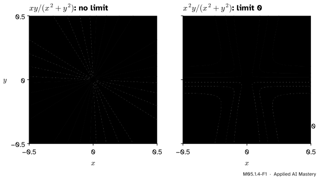
M05.1.4-F1
Left: every level set of \({xy/(x^2 + y^2)}\) is a ray from the origin, so every value from \({-1/2}\) to \({1/2}\) occurs arbitrarily close to it. Right: the level sets of \({x^2y/(x^2 + y^2)}\) keep away from the origin, and in a small enough disc all values are small.
On the left the function is constant along every ray into the origin, but a different constant on each ray: 0 along the axes, \({1/2}\) along the diagonal \({y = x}\), \({-1/2}\) along \({y = -x}\). No single number can be its limit. On the right every level \({c \neq 0}\) stays outside a disc round the origin, so the closer you come, the smaller the values: the limit is 0.
Build it up
Step 1. Distance. In one variable, “close to \(a\)” meant \({\abs{x - a}}\) small. In \(\R^n\) the distance is the norm of the difference (M02.3.2), whose square is
Step 2. The open ball. The inputs within \(\delta\) of \(\vect{a}\) form the open ball\({\{\vect{x} : \norm{\vect{x} - \vect{a}} < \delta\}}\): an interval on the line, a disc in the plane, a solid sphere without its skin in space.
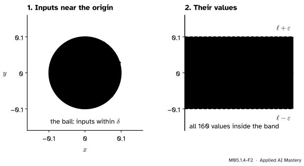
Step 3. The same tolerance game. M04.1.1 played it with a window round \(a\); now the window is a ball. A sceptic names a tolerance \({\varepsilon > 0}\) round the claimed limit \(\ell\). You must reply with a radius \({\delta > 0}\) such that every input in the ball, except perhaps \(\vect{a}\) itself, has its value within \(\varepsilon\) of \(\ell\).
M05.1.4-F2
The tolerance game for \({x^2y/(x^2 + y^2)}\) with \({\varepsilon = 0.1}\). The answer \({\delta = 0.1}\) works: every input in the ball (left) has its value inside the band (right).
Step 4. Paths. If \(f\) has limit \(\ell\), then along any path that runs into \(\vect{a}\) the values must tend to \(\ell\) too, because the path ends up inside every ball. Read backwards, this is a test for failure: two paths with two different limits prove that no limit exists.
The formal statement
NoteDefinitions: limit and continuity
Let \(f\) be defined at every point of some ball round \(\vect{a}\) in \(\R^n\), except perhaps at \(\vect{a}\) itself. The limit of \({f(\vect{x})}\) as \(\vect{x}\) tends to \(\vect{a}\) is \(\ell\), written \({\lim_{\vect{x} \to \vect{a}} f(\vect{x}) = \ell}\), if for every \({\varepsilon > 0}\) there is a \({\delta > 0}\) such that
\(f\) is continuous at \(\vect{a}\) if \(f\) is defined at \(\vect{a}\) and \({\lim_{\vect{x} \to \vect{a}} f(\vect{x}) = f(\vect{a})}\).
For \({n = 1}\) this is the definition of M04.1.1 word for word, since the norm of a number is its absolute value. Three results do the everyday work.
The two-path test. If \({\vect{r}(t)}\) is a path with \({\vect{r}(t) \neq \vect{a}}\) for \({t > 0}\) and \({\vect{r}(t) \to \vect{a}}\) as \({t \to 0}\), and \(f\) has limit \(\ell\) at \(\vect{a}\), then \({f(\vect{r}(t)) \to \ell}\). Why. Given \(\varepsilon\), take the \(\delta\) of the definition. Once \(t\) is small enough, \({\vect{r}(t)}\) lies in the ball of radius \(\delta\), and then \({\abs{f(\vect{r}(t)) - \ell} < \varepsilon}\).
The squeeze. Suppose \({\abs{f(\vect{x}) - \ell} \le C\,\norm{\vect{x} - \vect{a}}}\) for a constant \({C > 0}\) and every \(\vect{x}\) with \({0 < \norm{\vect{x} - \vect{a}} < \rho}\). Then the limit is \(\ell\): given \(\varepsilon\), take \(\delta\) to be the smaller of \({\varepsilon / C}\) and \(\rho\). Then \({0 < \norm{\vect{x} - \vect{a}} < \delta}\) gives \({\abs{f(\vect{x}) - \ell} < C\delta \le \varepsilon}\). (In this lesson’s examples the bound holds everywhere, so \({\delta = \varepsilon / C}\) will do.)
Building continuous functions. If \(f\) and \(g\) are continuous at \(\vect{a}\), so are \({f + g}\), \({fg}\) and, when \({g(\vect{a}) \neq 0}\), \({f / g}\). If \(g\) is continuous at \(\vect{a}\) and \(\phi\), a function of one variable, is continuous at \({g(\vect{a})}\), then \({\phi \circ g}\) is continuous at \(\vect{a}\). The proofs repeat those of the limit laws of M04.1.2 with the norm in place of the absolute value; the sum rule is written out below, and the others are stated without proof, as in M04.1.
Start from the coordinate functions \({\vect{x} \mapsto x_i}\). They are continuous by the squeeze with \({C = 1}\), because one coordinate never differs by more than the whole distance:
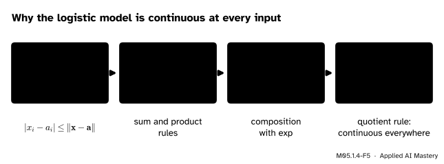
Sums and products of coordinates give every polynomial, so the running loss and every linear model are continuous everywhere. Composing with \(\exp\), adding 1 and dividing (the bottom is never 0) gives the sigmoid of any linear score. The same steps show that softmax and the mean squared error are continuous everywhere, and the log loss wherever its probabilities lie strictly between 0 and 1.
M05.1.4-F5
Continuity is assembled from pieces. Each arrow is one of the rules above, and the result is that the logistic model is continuous at every input.
Go deeper: the sum rule, with every step
Let \(f\) and \(g\) be continuous at \(\vect{a}\), and let \({\varepsilon > 0}\). Use the definition for each with the tolerance \({\varepsilon/2}\): there is a \({\delta_1}\) such that \({\norm{\vect{x} - \vect{a}} < \delta_1}\) gives \({\abs{f(\vect{x}) - f(\vect{a})} < \varepsilon/2}\), and a \({\delta_2}\) that does the same for \(g\). Take \(\delta\) to be the smaller of the two. Then both hold at once, and by the triangle inequality
No limit: \({f(x, y) = xy/(x^2 + y^2)}\) at the origin.
Two paths. On the \(x\) axis, \({y = 0}\) and \({f(x, 0) = 0/x^2 = 0}\) for every \({x \neq 0}\). On the diagonal, \({f(x, x) = x^2 / 2x^2 = 1/2}\). Two paths, two limits, so by the two-path test there is no limit, whatever value is assigned at the origin, and \(f\) cannot be continuous there.
Every ray at once. Write the point in polar form, \({x = r\cos\theta}\) and \({y = r\sin\theta}\) with \({r > 0}\). Then \({x^2 + y^2 = r^2}\) and
using \({2\sin\theta\cos\theta = \sin 2\theta}\). The value depends on the angle only: along each ray it is a constant, and the constants run through every number from \({-1/2}\) to \({1/2}\). Its level sets are the rays of the anchor figure.
Limit 0: \({g(x, y) = x^2 y/(x^2 + y^2)}\) at the origin.
Squeeze. Since \({x^2 \le x^2 + y^2}\), the fraction \({x^2/(x^2 + y^2)}\) is at most 1, so
This is the squeeze with \({\ell = 0}\) and \({C = 1}\), so \({\delta = \varepsilon}\) wins the tolerance game: \({\lim_{(x, y) \to (0, 0)} g = 0}\). Setting \({g(0, 0) = 0}\) makes \(g\) continuous everywhere. In polar form \({g = r\cos^2\theta\sin\theta}\), so on every ray it runs straight into 0.
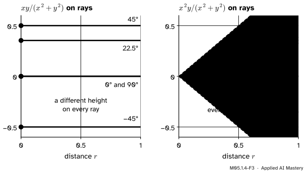
M05.1.4-F3
Both functions sliced along rays into the origin (lesson 3), as functions of the distance \(r\). Left: a different constant on each ray. Right: every slice is squeezed into the wedge \({\abs{g} \le r}\).
Code
A table along many paths into the origin, for both functions.
import numpy as npf =lambda x, y: x * y / (x**2+ y**2)g =lambda x, y: x**2* y / (x**2+ y**2)r =10.0**-np.arange(1, 7) # distances 0.1, 0.01, ..., 0.000001angles = np.radians([0, 22.5, 45, 90, 135, 200])for a in angles: xs, ys = r * np.cos(a), r * np.sin(a)print(f"{np.degrees(a):6.1f}° f: {f(xs, ys)[-1]: .4f} g: {g(xs, ys)[-1]: .2e}")
Along every ray \(f\) keeps its own value, \({\tfrac12\sin 2\theta}\), while \(g\) shrinks with \(r\). The table agrees with the proofs, but it does not replace them: it looks at six distances on six rays, and a limit is a statement about every point of a ball. The next function shows why that matters. Let \({p(x, y) = x^2 y/(x^4 + y^2)}\).
p =lambda x, y: x**2* y / (x**4+ y**2)for m in (0.5, 1, 3, -2):print(f"line y = {m:4}x: ", np.round(p(r, m * r), 6))print("parabola y = x^2:", p(r, r**2))
line y =  0.5x:   [1.92308e-01 1.99920e-02 2.00000e-03 2.00000e-04 2.00000e-05 2.00000e-06]
line y =    1x:   [9.901e-02 9.999e-03 1.000e-03 1.000e-04 1.000e-05 1.000e-06]
line y =    3x:   [3.3296e-02 3.3330e-03 3.3300e-04 3.3000e-05 3.0000e-06 0.0000e+00]
line y =   -2x:   [-4.9875e-02 -5.0000e-03 -5.0000e-04 -5.0000e-05 -5.0000e-06 -0.0000e+00]
parabola y = x^2: [0.5 0.5 0.5 0.5 0.5 0.5]
Along every straight line \(p\) dwindles to 0, yet along the parabola \({y = x^2}\) it is exactly \({1/2}\) at every distance. A table of straight lines would have voted for the limit 0.
Explore
This module’s interactive, the level-set explorer, lives in lesson M05.1.3. Its functions are all continuous, so there every level set is a clean curve; compare them with the fan of rays in this lesson’s anchor figure.
Pitfalls
M05.1.4-F4
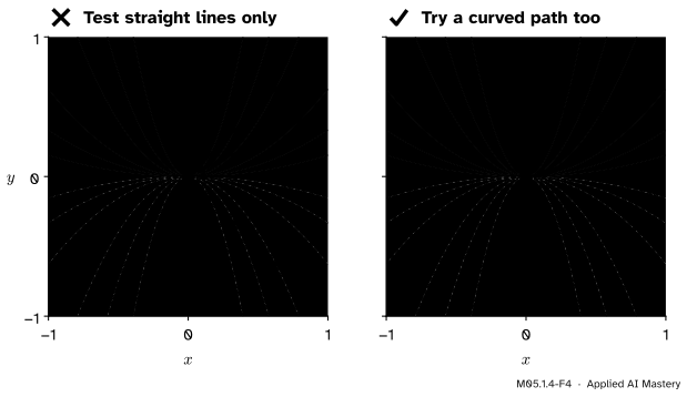
Wrong beside right. The level sets of \({x^2y/(x^4 + y^2)}\) are parabolas through the origin, so every straight line cuts across them towards level 0, while the parabola \({y = x^2}\) stays on level \({1/2}\).
“Every straight line into the point gives the same value, so that is the limit.”
Straight lines are only some of the paths. For \({x^2y/(x^4 + y^2)}\), the line \({y = mx}\) gives \({mx/(x^2 + m^2)}\), which tends to 0, but the parabola \({y = kx^2}\) gives \({k/(1 + k^2)}\) all the way in, \({1/2}\) for \({k = 1}\). Agreement along paths can only suggest a limit; a proof needs the ball, as in a squeeze.
“The function is defined at the point, so it is continuous there.”
Giving \({xy/(x^2 + y^2)}\) the value 0 at the origin defines it there, and makes both partial derivatives exist, but values of \({1/2}\) remain arbitrarily close by. Continuity asks that the nearby values approach the value at the point, from every direction at once.
“The table converges, so the limit exists.”
A table samples a few paths at a few distances. It can reveal that a limit fails (two rows heading for different values), but it cannot prove that one exists. Use it to guess, then prove.
Check yourself
Recall
1. State the definition of \({\lim_{\vect{x} \to \vect{a}} f(\vect{x}) = \ell}\).
Show answer
For every \({\varepsilon > 0}\) there is a \({\delta > 0}\) such that \({0 < \norm{\vect{x} - \vect{a}} < \delta}\) implies \({\abs{f(\vect{x}) - \ell} < \varepsilon}\).
2. What is an open ball, and what is it in the plane?
Show answer
The set of points within a distance \(\delta\) of \(\vect{a}\), \({\norm{\vect{x} - \vect{a}} < \delta}\); in the plane, a disc without its edge.
3. How do you show that a limit does not exist?
Show answer
Find two paths into the point along which the function tends to different values (or one along which it has no limit).
4. What is \({xy/(x^2 + y^2)}\) in polar form, and what does that say?
Show answer
\({\tfrac12\sin 2\theta}\): it depends on the angle only, so it is constant on each ray, with different constants on different rays, and has no limit at the origin.
5. Why is the sigmoid of a linear score, \({\sigma(\vect{w}\T\vect{x} + b)}\), continuous?
Show answer
The score is a polynomial in the coordinates, which are continuous; exponentials, sums and a quotient whose bottom \({1 + e^{-z}}\) is never 0 keep continuity, and so does composition.
Exercises
1.★ Show that \({(x^2 - y^2)/(x^2 + y^2)}\) has no limit at the origin.
Show solution
On the \(x\) axis, \({y = 0}\), the value is \({x^2/x^2 = 1}\). On the \(y\) axis it is \({-y^2/y^2 = -1}\). Two paths, two limits, so there is no limit. (In polar form it is \({\cos 2\theta}\).)
2.★★ Prove that \({(x^3 + y^3)/(x^2 + y^2)}\) tends to 0 at the origin, and give a \(\delta\) for \({\varepsilon = 0.01}\).
Show solution
Write \({r = \sqrt{x^2 + y^2}}\). Since \({\abs{x} \le r}\), \({\abs{x}^3 = \abs{x}\,x^2 \le r\,x^2}\), and likewise \({\abs{y}^3 \le r\,y^2}\). So
and dividing by \({x^2 + y^2 = r^2}\) gives \({\abs{f} \le r}\). By the squeeze with \({C = 1}\), the limit is 0, and \({\delta = \varepsilon = 0.01}\) works.
3.★★★ In \(\R^3\), decide whether \({xyz/(x^2 + y^2 + z^2)}\) and \({xy/(x^2 + y^2 + z^2)}\) have limits at the origin.
Show solution
Let \({r = \norm{(x, y, z)}}\). Each coordinate is at most \(r\) in size, so \({\abs{xyz} \le r^3}\) and
By the squeeze the first tends to 0. For the second, on the line \({x = y}\), \({z = 0}\) it is \({x^2/(2x^2) = 1/2}\), while on the \(x\) axis it is 0: two paths, two limits, so it has no limit.
Summary card
A limit in several variables must hold on a whole ball, so every path in must agree.
M05.1.4-F1
A fan of values, and a squeeze.
Limit: every tolerance \(\varepsilon\) has a ball of radius \(\delta\) whose values (bar \(\vect{a}\)) lie within \(\varepsilon\) of \(\ell\).
No limit: two paths with different limits; \({xy/(x^2 + y^2) = \tfrac12\sin 2\theta}\).
Continuity: sums, products, quotients and compositions of continuous functions.
Sources and next steps
Sources. Each was opened and checked against this lesson on 15 November 2026.
Gilbert Strang and Edwin Herman, Calculus Volume 3 (OpenStax), Section 4.2: the limit of a function of two variables defined with a \(\delta\) disk (an open disk of radius \(\delta\)), Example 4.9, where \({2xy/(3x^2 + y^2)}\) gives 0 along \({y = 0}\) and \({1/2}\) along \({y = x}\), and \({4xy^2/(x^2 + 3y^4)}\) gives 0 along every line \({y = kx}\) but 1 along the parabola \({x = y^2}\), Theorems 4.2 and 4.4 on sums and compositions of continuous functions, and \(\delta\) balls for three or more variables.
Gilbert Strang and Edwin Herman, Calculus Volume 3 (OpenStax), Section 4.1: functions of several variables and their domains.
Next. The module is complete. Module M05.2 differentiates functions of many inputs and finds that \({xy/(x^2 + y^2)}\), with partial derivatives but no limit, is the standard warning that partial derivatives alone do not make a function differentiable.