When no formula solves a differential equation, follow its slope for a short time and look again. Derive Euler’s method from the tangent line, run it by hand on y’ = y, watch the error shrink in step with the step size, and find that on a loss it is gradient descent, with the same step-size limit.
Derive Euler’s step from the linear approximation, and carry out several steps by hand.
Explain why the error of Euler’s method at a fixed time shrinks in proportion to the step, and prove the bound (e/2) times the step for y’ = y.
Show that Euler’s method on the gradient flow w’ = -L’(w) is gradient descent with learning rate equal to the step, and derive its stability limit of 2/15 on the running loss.
Write Euler’s method from scratch, and solve the same equations with scipy.integrate.solve_ivp.
In review. The maths and code on this page are checked by automated tests on every change, but an independent reader has not signed it off yet. Spot a mistake or a confusing step? Tell us.
The question
Most differential equations have no formula for their solution. The gradient flow of a neural network’s loss is one of them, and yet every training run traces out a path. How do you follow a rule about rates that you cannot solve? And why does training blow up when the learning rate is too large, even though the smooth curve it imitates never does?
From the last lesson
1. Solve \({y' = t\,y}\) with \({y(0) = 1}\).
Show answer
\({y = e^{t^2/2}}\), by separating: \({dy/y = t\,dt}\).
2. Which equilibrium of \({y' = y\,(1 - y)}\) is stable, and why?
Show answer
\({y = 1}\): the rate is positive just below it and negative just above, so solutions move towards it.
Intuition
Stand at the starting point. The equation tells you the slope there. Walk along that straight line for a short time \({\Delta t}\), and you will be close to the true solution, though not on it. Now ask the equation for the slope at the new point, and walk again. The path is a chain of straight steps that bends as the slopes change: Euler’s method.
M04.9.4-F1
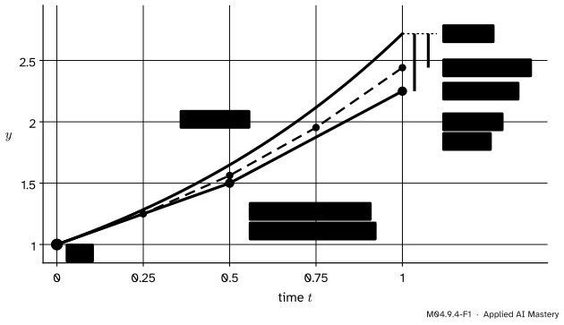
Euler’s method on \({y' = y}\) from \({y(0) = 1}\). Two steps of 0.5 reach 2.25 and four steps of 0.25 reach 2.441, against the exact \({e \approx 2.718}\). Halving the step brought the path closer.
Build it up
Step 1. One step is the tangent line. The linear approximation of M04.2.2 says that for a small \({\Delta t}\), \({y(t + \Delta t) \approx y(t) + y'(t)\,\Delta t}\). A differential equation tells us \({y'(t) = f(t, y(t))}\), so
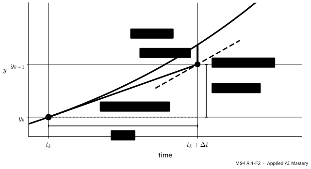
One Euler step. Follow the tangent for a time \({\Delta t}\): the rise is \({\Delta t}\) times the slope. The new point misses the curve by a small error, and the slope there is new.
Step 2. Repeat. Start at \({(t_0, y_0)}\), take the step, and treat the new point as a fresh start. The steps are counted by \(k\):
Step 3. On y′ = y, each step multiplies. With \({f(t, y) = y}\), a step is \({y_{k+1} = y_k + \Delta t\,y_k = (1 + \Delta t)\,y_k}\). From \({y_0 = 1}\), \(n\) steps of \({\Delta t = 1/n}\) reach \({t = 1}\) with
\[
y_n = \Big(1 + \frac{1}{n}\Big)^{n} .
\]
These are the compound-interest numbers of M01.4.2, 2, 2.25, 2.4414 and so on, which settle towards \(e\). Euler’s method on \({y' = y}\) is compound interest.
Step 4. Why the error is proportional to the step. Each step misses by the error of a tangent line, which shrinks like \({\Delta t^2}\) (M04.2.2). Reaching a fixed time \(T\) takes \({T/\Delta t}\) steps, so the total error is roughly
Halve the step and the error roughly halves, but the work doubles. This is a rough count, because an early error is carried along by later steps; the formal statement proves a sharp bound for \({y' = y}\).
Step 5. On a loss, Euler’s method is gradient descent. Apply it to the gradient flow \({w' = -L'(w)}\) of lesson M04.9.2:
That is the gradient-descent update of M04.4.4, with learning rate \({\eta = \Delta t}\). Training a model by gradient descent is following its gradient flow by Euler’s method.
The formal statement
NoteDefinition: Euler’s method
For the initial value problem \({y' = f(t, y)}\), \({y(t_0) = y_0}\), choose a step \({\Delta t > 0}\) and repeat, for \({k = 0, 1, 2, \ldots}\),
The error is first order. For an equation whose \(f\) is smooth, the error at a fixed time is at most a constant times \({\Delta t}\). Methods with this property are called first order. The general proof needs tools beyond this course, but for \({y' = y}\) the bound can be proved by hand.
NoteResult: the error of Euler’s method on y′ = y
With \({y(0) = 1}\) and \(n\) steps of \({\Delta t = 1/n}\), Euler’s method gives \({(1 + \Delta t)^{1/\Delta t}}\) at \({t = 1}\), and
\[
0 \le e - (1 + \Delta t)^{1/\Delta t} \le \frac{e}{2}\,\Delta t .
\]
Go deeper: proof of the error bound
Write \({h = \Delta t > 0}\). Two inequalities about \(\ln\) hold for every \({h \ge 0}\):
\[
h - \frac{h^2}{2} \le \ln(1 + h) \le h .
\]
For the right one, \({\psi(h) = h - \ln(1 + h)}\) has \({\psi(0) = 0}\) and \({\psi'(h) = 1 - 1/(1 + h) \ge 0}\), so \(\psi\) never decreases and stays at least 0. For the left one, \({\phi(h) = \ln(1 + h) - h + h^2/2}\) has \({\phi(0) = 0}\) and
so \(\phi\) stays at least 0 too. Divide by \(h\) and exponentiate, which keeps the order:
\[
e^{1 - h/2} \le (1 + h)^{1/h} \le e .
\]
The right half says the error is at least 0. For the left half, \({e^{-x} \ge 1 - x}\) for \({x \ge 0}\) (the same argument with \({e^{-x} - 1 + x}\), whose derivative \({1 - e^{-x}}\) is never negative), so
\[
\begin{aligned}
e - (1 + h)^{1/h} &\le e\,\big(1 - e^{-h/2}\big) \\
&\le e \cdot \frac{h}{2} .
\end{aligned}
\]
The bound also shows that Euler’s method always falls short on \({y' = y}\): each step follows a tangent line, and the exponential curves upward away from it.
Stability. Euler’s method can fail in a way the exact solution never does. Take an approach to a level, \({y' = -\lambda\,(y - c)}\) with a rate \({\lambda > 0}\) (we write \(\lambda\) here, because \(k\) now counts steps). Subtracting \(c\) from both sides of an Euler step gives
\[
\begin{aligned}
y_{k+1} - c &= (y_k - c) - \lambda\,\Delta t\,(y_k - c) \\
&= (1 - \lambda\,\Delta t)\,(y_k - c) .
\end{aligned}
\]
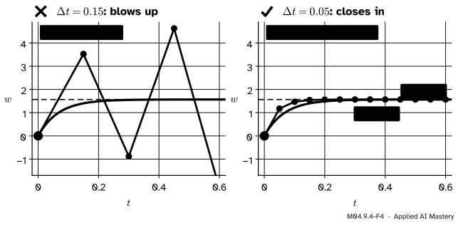
Every step multiplies the distance to \(c\) by \({m = 1 - \lambda\,\Delta t}\). The distance shrinks to 0 exactly when \({-1 < m < 1}\), that is when \({0 < \Delta t < 2/\lambda}\). For \({\Delta t < 1/\lambda}\) the factor is positive and the path closes in from one side, like the exact solution. For \({1/\lambda < \Delta t < 2/\lambda}\) the factor is negative and the path jumps across the level each step, though it still closes in. For \({\Delta t > 2/\lambda}\) every jump is longer than the last and the path blows up, while the exact solution \({c + (y_0 - c)\,e^{-\lambda t}}\) converges for every \({\lambda > 0}\).
On the running loss, \({\lambda = 15}\) and \({c = 47/30}\). The limits are \({1/15 \approx 0.067}\) and \({2/15 \approx 0.133}\): exactly the learning-rate limits of ML01.5.3, seen now as the stability limit of a method for differential equations. The tea of M04.9.2, with \({\lambda = k \approx 0.056}\) per minute, allows steps of up to about 36 minutes.
Frontier note: a residual network is Euler's method
A residual network updates a hidden state layer by layer as \({h_{t+1} = h_t + f(h_t, \theta_t)}\), where \(t\) counts the layers. Chen, Rubanova, Bettencourt and Duvenaud (2018) point out that this is an Euler step with \({\Delta t = 1}\) (their equation 1). Taking more layers and smaller steps leads to a neural ordinary differential equation, \({dh/dt = f(h(t), t, \theta)}\) (their equation 2), whose output is computed by an ODE solver of the kind called below. Lesson M12.7 builds one.
Worked example
Run Euler’s method on \({y' = y}\) from \({y(0) = 1}\) to \({t = 1}\), with steps of 0.5 and then 0.25, and compare with \(e\). Then take three steps of gradient flow on the running loss with \({\Delta t = 0.1}\).
Steps of 0.5. The slope at the start is \({f(0, 1) = 1}\), so \({y_1 = 1 + 0.5 \times 1 = 1.5}\). The slope there is 1.5, so \({y_2 = 1.5 + 0.5 \times 1.5 = 2.25}\). The error is \({e - 2.25 \approx 0.468}\).
Steps of 0.25. Each step multiplies by 1.25: 1.25, 1.5625, 1.9531, 2.4414. The error is \({e - 2.4414 \approx 0.277}\).
M04.9.4-F3
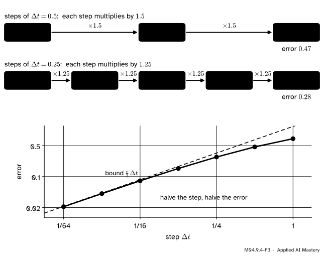
The worked example. Each step of Euler’s method on \({y' = y}\) multiplies by \({1 + \Delta t}\). Below, the error at \({t = 1}\) for steps from 1 down to \({1/64}\): halving the step about halves the error, and the bound \({\frac{e}{2}\,\Delta t}\) is nearly met.
Halving the step cut the error from 0.468 to 0.277, by a factor of 0.59. Halving again gives factors of 0.55, 0.53 and 0.51, settling at one half: the error is proportional to the step, close to \({\frac{e}{2}\,\Delta t \approx 1.36\,\Delta t}\) for small steps.
Gradient flow with \({\Delta t = 0.1}\). With \({L'(w) = 15w - 23.5}\) and \({w_0 = 0}\):
The distances to \({47/30 \approx 1.567}\) are \({-1.567}\), 0.783, \({-0.392}\) and 0.196: each is \({-0.5}\) times the last, because \({m = 1 - 15 \times 0.1 = -0.5}\). The path jumps across the minimum at every step, while the exact flow never crosses it.
Code
Euler’s method from scratch is a loop of two lines:
import mathdef euler(f, t0, y0, dt, steps):"""Follow the slope f(t, y) for a time dt, then look again; repeat `steps` times.""" t, y = t0, y0 path = [(t, y)]for _ inrange(steps): y = y + dt * f(t, y) t = t + dt path.append((t, y))return pathgrow =lambda t, y: yfor n in (2, 4, 8, 16, 32, 64): end = euler(grow, 0.0, 1.0, 1/ n, n)[-1] error = math.e - end[1]print(f"dt = 1/{n:<3} y(1) = {end[1]:.6f} error {error:.6f} error/dt {error * n:.4f}")
On the gradient flow of the running loss, Euler’s method and gradient descent produce the same numbers, and the step decides the behaviour:
slope =lambda w: 15* w -23.5flow =lambda t, w: -slope(w)for dt in (0.05, 0.1, 0.15): ws = [w for _, w in euler(flow, 0.0, 0.0, dt, 4)]print(f"dt = {dt:<4} w = {[round(w, 4) for w in ws]} factor {1-15* dt:+.2f}")w, eta, descent =0.0, 0.05, [0.0]for _ inrange(4): w = w - eta * slope(w) # the update of M04.4.4 descent.append(w)print("gradient descent, eta = 0.05:", [round(w, 4) for w in descent])
The library’s solver is scipy.integrate.solve_ivp. Its default method, RK45, is a Runge–Kutta method of order 5(4): it estimates its own error at every step and keeps that estimate within the tolerances rtol and atol, choosing the times itself:
import numpy as npfrom scipy.integrate import solve_ivpfor rtol, atol in ((1e-3, 1e-6), (1e-10, 1e-12)): sol = solve_ivp(lambda t, y: y, (0, 1), [1.0], rtol=rtol, atol=atol)print(f"rtol = {rtol:.0e}: y(1) = {sol.y[0, -1]:.10f}, error {abs(sol.y[0, -1] - math.e):.1e}, "f"{sol.nfev} evaluations of f")logi = solve_ivp(lambda t, y: y * (1- y), (0, 4), [0.5], t_eval=[0, 2, 4], rtol=1e-10, atol=1e-12)print("logistic from 1/2 at t = 0, 2, 4:", np.round(logi.y[0], 6))print("the sigmoid at the same times: ", np.round(1/ (1+ np.exp(-logi.t)), 6))
rtol = 1e-03: y(1) = 2.7183269995, error 4.5e-05, 14 evaluations of f
rtol = 1e-10: y(1) = 2.7182818285, error 5.4e-11, 170 evaluations of f
logistic from 1/2 at t = 0, 2, 4: [0.5      0.880797 0.982014]
the sigmoid at the same times:    [0.5      0.880797 0.982014]
With its default tolerances solve_ivp reaches \(e\) to within \({10^{-4}}\) after fewer than 30 evaluations of \(f\). Euler’s method, with its error of about \({1.36\,\Delta t}\), needs more than ten thousand steps for that. With the tight tolerances the solver’s error falls below \({10^{-9}}\) for fewer than 300 evaluations, where Euler’s method would need over a billion steps. Better solvers are the subject of M12.2.
Explore
M04.9-X1
Slope field and Euler stepper
Choose an equation, then click on the slope field (or use the sliders) to set the start, and change the step. Try \({y' = y}\) with steps of 0.5 and 0.25 to see the worked example, then gradient flow with steps either side of \({1/15}\) and \({2/15}\).
Pitfalls
M04.9.4-F4
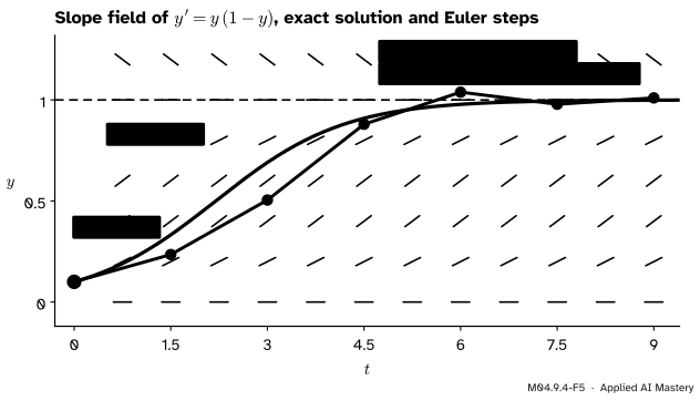
Wrong beside right on the gradient flow of the running loss. The flow itself is the same smooth curve in both panels; only the step differs.
“If the true solution settles, the Euler path settles too.”
The gradient flow of the running loss settles for any start, yet Euler’s method with \({\Delta t = 0.15}\) multiplies the distance by \({-1.25}\) at every step and blows up. The step must be short compared with the fastest rate in the equation: here \({\Delta t < 2/15}\). A training run that diverges has broken this limit.
“A smaller step is always worth it.”
Halving the step halves the error and doubles the work. To get \(e\) to six decimal places Euler’s method needs over a million steps, which is why real solvers use better methods than one tangent line per step.
“The errors of the steps cancel out.”
On \({y' = y}\) every step lands below the curve through its starting point, because the exponential curves upward away from its tangent lines. The errors all point the same way and add up, which is why the Euler values 2.25 and 2.4414 both fall short of \(e\).
2. Which approximation from M04.2 does each step use?
Show answer
The tangent line, or linear approximation: \({y(t + \Delta t) \approx y(t) + y'(t)\,\Delta t}\).
3. What does Euler’s method give for \({y' = y}\), \({y(0) = 1}\), with four steps of 0.25, and what is the error?
Show answer
\({1.25^4 \approx 2.4414}\), against \({e \approx 2.7183}\): an error of about 0.277.
4. What happens to the error at a fixed time when the step is halved?
Show answer
It roughly halves, because Euler’s method is first order: its error is proportional to the step.
5. What is Euler’s method on \({w' = -L'(w)}\), and what step does the running loss allow?
Show answer
Gradient descent with learning rate \({\eta = \Delta t}\). It converges only for \({\Delta t < 2/15}\), and without overshooting only for \({\Delta t \le 1/15}\).
Exercises
1.★ Take two Euler steps of 0.5 on \({y' = 1 - y}\) from \({y(0) = 0}\), and compare with the exact value \({1 - e^{-1}}\) at \({t = 1}\).
Show solution
\({y_1 = 0 + 0.5 \times (1 - 0) = 0.5}\) and \({y_2 = 0.5 + 0.5 \times (1 - 0.5) = 0.75}\). The exact value is \({1 - e^{-1} \approx 0.632}\), so Euler’s method overshoots by about 0.118. Here the curve bends downward, so each tangent line lies above it, the opposite of \({y' = y}\).
2.★★ The tea of M04.9.2 follows \({y' = -k\,(y - 20)}\) with \({k = \ln(7/4)/10}\) per minute and \({y(0) = 90}\). Use Euler’s method with steps of 10 minutes to estimate \({y(20)}\), and compare with the exact 42.86 °C. What happens with steps of 40 minutes, and why?
Show solution
Each step multiplies the gap above 20 by \({m = 1 - 10k \approx 0.4404}\). After two steps the gap is \({70 \times 0.4404^2 \approx 13.58}\), so \({y(20) \approx 33.6}\) °C: far too cold, because \({10k}\) is not small. The exact gap is \({70\,(4/7)^2 \approx 22.86}\). With steps of 40 minutes, \({m = 1 - 40k \approx -1.24}\): the first step gives a gap of \({-86.7}\), a tea at \({-66.7}\) °C, and each later jump is longer. The step is above \({2/k \approx 35.7}\) minutes, the stability limit.
3.★★★ Euler’s method on the logistic equation is \({y_{k+1} = y_k + \Delta t\,y_k(1 - y_k)}\). Writing \({y_k = 1 + d_k}\), show that \({d_{k+1} = (1 - \Delta t)\,d_k - \Delta t\,d_k^2}\). For which steps do paths close to 1 settle there, and when do they jump across it? Check with \({\Delta t = 1.5}\) from \({y_0 = 0.1}\).
Show solution
With \({y = 1 + d}\), \({y\,(1 - y)} = {(1 + d)(-d)} = {-d - d^2}\). So
Near 1 the square is tiny and \({d_{k+1} \approx (1 - \Delta t)\,d_k}\): the stability rule with \({\lambda = 1}\). Paths near 1 settle when \({0 < \Delta t < 2}\), and they jump across 1 at each step when \({\Delta t > 1}\). With \({\Delta t = 1.5}\) from 0.1 the path is 0.235, 0.505, 0.880, 1.038, 0.979, 1.010, 0.995: across 1 and back, each distance about \({-0.5}\) times the last, as \({1 - 1.5 = -0.5}\) predicts.
Summary card
Follow the slope for \({\Delta t}\), then look again: Euler’s method is the tangent line, repeated.
Error at a fixed time is proportional to \({\Delta t}\); on \({y' = y}\) it is at most \({\frac{e}{2}\,\Delta t}\).
Gradient descent is Euler’s method on \({w' = -L'(w)}\) with \({\eta = \Delta t}\).
Stability. On \({y' = -\lambda\,(y - c)}\) each step multiplies the distance by \({1 - \lambda\,\Delta t}\); it settles only if \({\Delta t < 2/\lambda}\).
Sources and next steps
Sources. Each was opened and checked against this lesson on 12 November 2026.
Gilbert Strang and Edwin Herman, Calculus Volume 2 (OpenStax), Section 4.2: Euler’s method for \({y' = f(x, y)}\) (Theorem 4.1, Equation 4.2) with step size \(h\), and a comparison of steps of 0.5 and 0.25 (Figure 4.14).
Matthew Boelkins, Active Calculus, Section 7.3: Euler’s method with the step \({\Delta t}\), as following tangent lines, and the statement that its error at a point is proportional to \({\Delta t}\), with a table for \({y' = y}\) in which halving the step roughly halves the error.
Jiří Lebl, Notes on Diffy Qs, Section 1.7: Euler’s method as a first-order method (each halving of the step about halves the error), numerical instability with too large a step (Exercise 1.7.6), and Runge–Kutta methods.
SciPy developers, scipy.integrate.solve_ivp (SciPy 1.18 reference): the call \({\text{fun}(t, y)}\), the default method RK45, an explicit Runge–Kutta method of order 5(4), and the default tolerances 1e-3 and 1e-6. The RK45 page adds that its local error estimates are kept below atol + rtol * abs(y).
Ricky T. Q. Chen, Yulia Rubanova, Jesse Bettencourt and David Duvenaud, Neural Ordinary Differential Equations, NeurIPS 2018. Section 1 presents the residual update (equation 1) as an Euler discretisation of a continuous transformation, and the neural ODE (equation 2).
Next. This completes the module. M04.10 Partial derivatives, a first look moves from one input to two. Solvers that take larger, smarter steps are M12.2, and the stability of equations with several unknowns is M12.3.