Partial derivatives: the slope when one input moves
Freeze one input of a function of two variables and an ordinary curve is left, with an ordinary slope. That slope is a partial derivative. Find it from the definition and by the rules of differentiation, and check it numerically.
Define the two partial derivatives of f(x, y) as limits of difference quotients in which one input stands still.
Compute partial derivatives from the definition and by the rules of differentiation, treating the frozen input as a constant.
Read a partial derivative as the slope of a slice through the surface.
Differentiate the squared error of one example with respect to the slope and the intercept with the chain rule.
Check partial derivatives with central differences and with numpy.gradient, knowing which output belongs to which input.
In review. The maths and code on this page are checked by automated tests on every change, but an independent reader has not signed it off yet. Spot a mistake or a confusing step? Tell us.
The question
Training asks one question over and over: if I nudge this parameter a little, how much does the loss change? With one parameter the answer is the derivative \({L'(w)}\) (M04.2.2). The loss \({L(w, b)}\) has two parameters. Nudge only \(w\) and the loss changes at one rate; nudge only \(b\) and it changes at another. What are those two rates, and how are they computed?
From the last lesson
1. What do you get when you freeze \({y = 1}\) in \({f(x, y) = x^2 + 2y^2}\)?
Show answer
The slice \({f(x, 1) = x^2 + 2}\), an ordinary function of \(x\) whose graph is a parabola.
2. Contour lines at equal steps of height lie close together in one part of a map. What does that tell you?
Show answer
The ground is steep there: the height changes a lot over a short distance.
Intuition
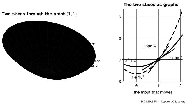
Stand at the point \({(1, 1)}\) of the running bowl, \({f(x, y) = x^2 + 2y^2}\), where the height is 3. Walk east, so that \(x\) grows and \(y\) stays at 1. You follow the slice \({y = 1}\), the parabola \({x^2 + 2}\), and the ground rises at its slope, 2. Walk north instead, so that \(y\) grows and \(x\) stays at 1. Now you follow the slice \({x = 1}\), the curve \({1 + 2y^2}\), which rises at slope 4.
M04.10.2-F1
One point, two slices, two slopes. With \(y\) frozen at 1 the bowl rises at slope 2 as \(x\) moves; with \(x\) frozen at 1 it rises at slope 4 as \(y\) moves.
The same point has two slopes, one for each input. Each is a partial derivative: the derivative of \(f\) with respect to one input while the other is held still. The slopes differ because the ground is steeper along \(y\), as the crowded contour lines of lesson 1 showed. Training needs exactly these numbers: the slope of a loss along \(w\) says how the loss responds to a nudge of \(w\) alone, and the slope along \(b\) how it responds to \(b\) alone.
Build it up
Step 1. Freeze \(y\). With \({y = 1}\) the bowl becomes \({g(x) = f(x, 1) = x^2 + 2}\), an ordinary function. By the power rule (M04.3.1) \({g'(x) = 2x}\), so \({g'(1) = 2}\).
Step 2. Freeze \(x\). With \({x = 1}\) it becomes \({k(y) = f(1, y) = 1 + 2y^2}\). Its derivative is \({k'(y) = 4y}\), so \({k'(1) = 4}\).
Step 3. Name the two slopes. They are written \({\pd{f}{x}(1, 1) = 2}\) and \({\pd{f}{y}(1, 1) = 4}\). The curly \({\partial}\), read “partial”, replaces the ordinary \(d\) to say that another input exists and is being held still.
Step 4. Every point at once. Freeze \(y\) at any value \(y_0\): the slice is \({x^2 + 2y_0^2}\). The second term is a constant, whose derivative is zero, so the slope is \(2x\). Hence \({\pd{f}{x} = 2x}\) at every point, and in the same way \({\pd{f}{y} = 4y}\).
The formal statement
NoteDefinition: partial derivatives
The partial derivatives of a function \(f\) of two variables at \((x, y)\) are
Each is the difference quotient of M04.2.1 with one input standing still, so \({\pd{f}{x}}\) is the slope of the slice through \((x, y)\) in the \(x\) direction. Inside the limit the frozen input is a plain number. So treat the frozen input as a constant, and every rule of M04.3 applies unchanged.
Example: \({f(x, y) = x^2 y + 3y}\). With respect to \(x\), \(y\) is a constant. The term \({x^2 y}\) is the constant \(y\) times \(x^2\), so its derivative is \({y \cdot 2x}\) by the constant-multiple rule. The term \({3y}\) contains no \(x\) at all; it is a constant, with derivative 0. So
\[
\pd{f}{x} = 2xy .
\]
With respect to \(y\), \(x\) is the constant. Now \({x^2 y}\) is the constant \(x^2\) times \(y\), with derivative \(x^2\), and \({3y}\) has derivative 3:
\[
\pd{f}{y} = x^2 + 3 .
\]
At \({(1, 2)}\) both equal 4.
Example: the squared error of one example. Take one data point \((x, y)\) and the line \({\hat{y} = wx + b}\). Here \(x\) and \(y\) are fixed numbers from the data; the inputs of the function are \(w\) and \(b\):
\[
e(w, b) = (wx + b - y)^2 .
\]
This is a square of the residual \({u = wx + b - y}\). By the chain rule (M04.3.4), the slope of \(u^2\) is \(2u\) times the slope of \(u\). With \(b\) held still, \(u\) changes \(x\) times as fast as \(w\) (the terms \(b\) and \(-y\) are constants). With \(w\) held still, \(u\) changes exactly as fast as \(b\). So
\[
\begin{aligned}
\pd{e}{w} &= 2(wx + b - y)\, x , \\
\pd{e}{b} &= 2(wx + b - y) .
\end{aligned}
\]
These are the terms that ML01.4.2 and ML01.5.2 average over the examples. For the point \({(3, 5)}\) at \({(w, b) = (1, 0)}\) the residual is \({3 - 5 = -2}\), so \({\pd{e}{w}} = {2 \cdot (-2) \cdot 3} = {-12}\) and \({\pd{e}{b} = -4}\). Raising \(w\) lowers this error three times as fast as raising \(b\), because \({x = 3}\).
Go deeper: two slopes do not see every direction
Let \({f(x, y) = xy/(x^2 + y^2)}\) away from the origin, and \({f(0, 0) = 0}\). On both axes \(f\) is 0, so both partial derivatives at the origin exist and equal 0. Yet on the line \({y = x}\), \({f(x, x)} = {x^2/(2x^2)} = {1/2}\) for every \({x \neq 0}\): arbitrarily close to the origin the height is \(\tfrac12\), so \(f\) is not even continuous there. Two slices see two directions only. Every function in this module is a polynomial, where nothing like this can happen; M05.2 treats the general case.
Worked example
Both slopes of the running bowl at \({(1, 1)}\), from the definition.
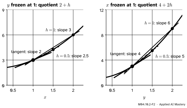
Along \(x\). Hold \({y = 1}\). Since \({(1 + h)^2 = 1 + 2h + h^2}\),
which tends to 4. A few values show both quotients closing in:
\(h\)
\({2 + h}\)
\({4 + 2h}\)
0.5
2.5
5
0.1
2.1
4.2
0.01
2.01
4.02
M04.10.2-F2
The worked example as a trace. On each slice the secant from \({(1, 1)}\) turns towards the tangent as \(h\) shrinks: slopes 3, 2.5, then 2 along \(x\); 6, 5, then 4 along \(y\).
By the rules, \({\pd{f}{x} = 2x}\) and \({\pd{f}{y} = 4y}\) give 2 and 4 at \({(1, 1)}\): the same answer in one line each.
Code
First from scratch: a central difference (M04.2.4) in each input, the other held still.
def partial_x(f, x, y, h=1e-5):return (f(x + h, y) - f(x - h, y)) / (2* h)def partial_y(f, x, y, h=1e-5):return (f(x, y + h) - f(x, y - h)) / (2* h)bowl =lambda x, y: x**2+2* y**2g =lambda x, y: x**2* y +3* yerror =lambda w, b: (w *3+ b -5) **2# one example, (x, y) = (3, 5)for name, func, at in [("bowl at (1, 1)", bowl, (1, 1)), ("x^2 y + 3y at (1, 2)", g, (1, 2)), ("error at (1, 0)", error, (1, 0))]:print(f"{name:21s}{partial_x(func, *at):10.6f}{partial_y(func, *at):10.6f}")
bowl at (1, 1)          2.000000   4.000000
x^2 y + 3y at (1, 2)    4.000000   4.000000
error at (1, 0)       -12.000000  -4.000000
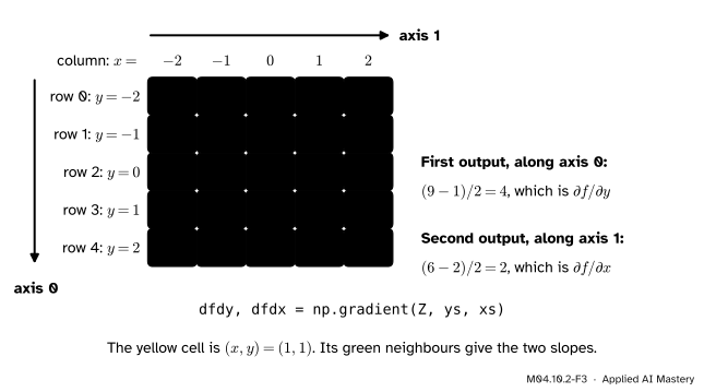
The printed slopes match the hand results to six decimals; further digits differ by rounding. Now the library version. np.gradient takes an array of heights on a grid, with the spacing along each axis, and returns one array of slopes per axis, in the order of the axes. Under np.meshgrid’s default the rows of the array follow \(y\), so axis 0 is \(y\) and the first output is the slope along \(y\).
M04.10.2-F3
How np.gradient reads the grid. Down the rows only \(y\) changes, so the first output is the slope in \(y\); along a row only \(x\) changes, so the second is the slope in \(x\).
import numpy as npxs = np.arange(-2.0, 3.0) # -2, -1, 0, 1, 2ys = np.arange(-2.0, 3.0)X, Y = np.meshgrid(xs, ys) # rows follow y, columns follow xZ = bowl(X, Y)dfdy, dfdx = np.gradient(Z, ys, xs) # axis 0 (y) first, then axis 1 (x)row, col =3, 3# ys[3] = 1 and xs[3] = 1print("at (1, 1): slope in x =", dfdx[row, col], " slope in y =", dfdy[row, col])print("slope in y down the column x = 1:", dfdy[:, col])
at (1, 1): slope in x = 2.0  slope in y = 4.0
slope in y down the column x = 1: [-6. -4.  0.  4.  6.]
Inside the grid the central difference of a quadratic is exact, so 2 and 4 come out exactly even with a spacing of 1. The column also shows the edges: there np.gradient can only look one way, and its one-sided differences give \(-6\) and 6 where the true slopes are \(-8\) and 8.
Explore
This module’s interactive, the slope compass, lives in lesson M04.10.3. Its two side panels are this lesson’s slices: drag the point and watch both tangent lines turn, with the two partial derivatives printed beside them.
Pitfalls
M04.10.2-F4
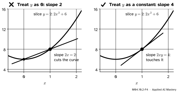
Wrong beside right, on the slice \({y = 2}\) of \({x^2 y + 3y}\). Dropping \(y\) gives a line that cuts the curve; keeping \(y\) as a constant gives the tangent.
“The frozen input is zero, so it drops out.”
It is held constant, not set to zero. In \({x^2 y + 3y}\) the derivative with respect to \(x\) is \({2xy}\), not \({2x}\): the \(y\) stays as a multiplier. Only a term with no \(x\) in it at all, like \({3y}\), drops out. The same slip in \({(wx + b - y)^2}\) would lose the factor \(x\) in \({\pd{e}{w}}\) and train with the wrong slope.
“A partial derivative tells me how \(f\) changes when I move.”
Only when you move along one axis. Step diagonally and both inputs change, so both slopes play a part; lesson 3 shows how they combine.
“np.gradient(Z) gives the slope along \(x\) first.”
It gives the slopes in the order of the array’s axes. With np.meshgrid’s default the rows follow \(y\), so the first output is the slope in \(y\). Write dfdy, dfdx = np.gradient(Z, ys, xs), and check one value by hand.
Check yourself
Recall
1. In words, what is \({\pd{f}{x}}\) at a point?
Show answer
The slope of the slice through the point with \(y\) held still: how fast \(f\) changes when only \(x\) moves.
2. Write \({\pd{f}{y}(x, y)}\) as a limit.
Show answer
The limit as \({h \to 0}\) of \({\big(f(x, y + h) - f(x, y)\big)/h}\).
3. What are the partial derivatives of \({x^2 + 2y^2}\), and their values at \({(1, 1)}\)?
Show answer
\({\pd{f}{x} = 2x}\) and \({\pd{f}{y} = 4y}\), so 2 and 4 at \({(1, 1)}\).
4. When you differentiate with respect to \(x\), how do you treat \(y\)?
Show answer
As a constant. Then all the rules of one-variable calculus apply.
5. What are the two partial derivatives of the squared error \({(wx + b - y)^2}\)?
Show answer
\({2(wx + b - y)\,x}\) with respect to \(w\), and \({2(wx + b - y)}\) with respect to \(b\).
Exercises
1.★ Find both partial derivatives of \({f(x, y) = 3x^2 - 2xy + y^3}\) and evaluate them at \({(1, 2)}\).
Show solution
With \(y\) constant: \({3x^2 \to 6x}\), \({-2xy \to -2y}\), \({y^3 \to 0}\), so \({\pd{f}{x} = 6x - 2y}\), which is \({6 - 4 = 2}\) at \({(1, 2)}\). With \(x\) constant: \({3x^2 \to 0}\), \({-2xy \to -2x}\), \({y^3 \to 3y^2}\), so \({\pd{f}{y} = -2x + 3y^2}\), which is \({-2 + 12 = 10}\).
2.★★ From the definition, find both partial derivatives of \({f(x, y) = x^2 y}\) at \({(1, 2)}\). One of the two quotients is the same for every \(h\): why?
Along \(y\), with \({x = 1}\): \({\big((2 + h) - 2\big)/h = 1}\) for every \(h\), so \({\pd{f}{y}(1, 2) = 1}\). With \(x\) frozen, \({x^2 y}\) is the straight line \(y\) times the constant 1, and a straight line’s secants all have its own slope. (By the rules: \({2xy = 4}\) and \({x^2 = 1}\).)
3.★★★ One example \({(x, y) = (2, 3)}\) gives the squared error \({e(w, b) = (2w + b - 3)^2}\). (a) Find both partial derivatives at \({(w, b) = (1, 0)}\). (b) Show that \({\pd{e}{w} = 2\,\pd{e}{b}}\) at every point, and say why. (c) Which lowers \(e\) more: raising \(w\) by 0.01, or raising \(b\) by 0.01?
Show solution
(a) The residual is \({u = 2 + 0 - 3 = -1}\). So \({\pd{e}{w}} = {2 \cdot (-1) \cdot 2} = {-4}\) and \({\pd{e}{b}} = {2 \cdot (-1)} = {-2}\).
(b) By the chain rule, \({\pd{e}{w} = 2u \cdot 2}\) and \({\pd{e}{b} = 2u}\), so the first is always twice the second. The factor is the example’s input, \({x = 2}\): moving \(w\) by one unit moves the prediction by 2, moving \(b\) by one unit moves it by 1.
(c) Raising \(w\) by 0.01 changes \(e\) by about \({-4 \times 0.01 = -0.04}\); raising \(b\), by about \({-0.02}\). So raising \(w\) helps twice as much. Exactly: \({e(1.01, 0)} = {(-0.98)^2} = {0.9604}\), a fall of 0.0396, and \({e(1, 0.01)} = {(-0.99)^2} = {0.9801}\), a fall of 0.0199.
Summary card
A partial derivative is the slope of a slice: how fast \(f\) changes when one input moves and the other stands still.
M04.10.2-F1
Two slices, two slopes.
\({\pd{f}{x}}\) is the limit of \({\big(f(x + h, y) - f(x, y)\big)/h}\); \({\pd{f}{y}}\) moves \(y\) instead.
Hold the other input constant and use the ordinary rules.
The bowl: \({\pd{f}{x} = 2x}\) and \({\pd{f}{y} = 4y}\), so 2 and 4 at \({(1, 1)}\).
Squared error: \({2(wx + b - y)\,x}\) and \({2(wx + b - y)}\).
dfdy, dfdx = np.gradient(Z, ys, xs) on a default meshgrid.
Sources and next steps
Sources. Each was opened and checked against this lesson on 12 November 2026.
Gilbert Strang and Edwin Herman, Calculus Volume 3 (OpenStax), Section 4.3: the partial derivatives as limits (Equations 4.12 and 4.13), the advice to treat every other variable as a constant, and the reading of \({\pd{f}{x}}\) as the slope of a tangent line parallel to the \(x\) axis.
Marc Peter Deisenroth, A. Aldo Faisal and Cheng Soon Ong, Mathematics for Machine Learning, Section 5.2: Definition 5.5, the partial derivative as a limit in which one variable changes and the others are kept constant, and Example 5.6, partial derivatives found with the chain rule.
NumPy 2.5 reference, numpy.gradient: central differences inside the array and one-sided differences at the edges, one output per axis, in the order of the axes (“the first array stands for the gradient in rows”).
Next.M04.10.3 The gradient puts the two slopes together into one arrow and finds the direction in which \(f\) climbs fastest.