The chain rule turns a composition into a product; substitution runs it backwards. Spot an inner function whose derivative is also present, rename it u, and the integral becomes one from the table. Worked on a polynomial, on the slope of the bell curve and on the sigmoid, whose integral is softplus.
Recognise an integrand of the form f(g(x)) g’(x) and choose the substitution u = g(x).
Derive the substitution rule from the chain rule and the fundamental theorem of calculus.
Change the limits of a definite integral to g(a) and g(b), and explain with slices why the area does not change.
Integrate x times the bell curve, and the sigmoid, by substitution, and check each antiderivative by differentiating it numerically.
In review. The maths and code on this page are checked by automated tests on every change, but an independent reader has not signed it off yet. Spot a mistake or a confusing step? Tell us.
The question
Softplus, \({\ln(1 + e^z)}\), is the smooth cousin of ReLU, and its slope is the sigmoid \({\sigma(z) = 1/(1 + e^{-z})}\). So the area under the sigmoid from 0 to 2 is the rise of softplus, \({\ln(1 + e^2) - \ln 2 \approx 1.434}\). But the table of antiderivatives (M04.6.3) has no line for \({1/(1 + e^{-z})}\). If nobody had told you about softplus, how could you have found it?
Intuition
Start with an integral that looks messy:
\[
\int_0^1 2x\,(x^2 + 1)^3\,dx .
\]
Look at its structure. Inside the cube sits an inner function, \({x^2 + 1}\). Outside, as a factor, sits \({2x}\), which is exactly the derivative of that inner function. Give the inner function a name of its own, \({u = x^2 + 1}\). As \(x\) runs from 0 to 1, \(u\) runs from 1 to 2.
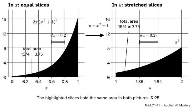
Now cut the \(x\)-interval into five equal slices and follow each slice to where \(u\) sends it.
M04.7.1-F1
The same area in two coordinates. Each equal slice in \(x\) (left) goes to a slice in \({u = x^2 + 1}\) (right). The \(u\)-slices are narrow near \({u = 1}\) and wide near \({u = 2}\), and the height changes by the opposite factor: matching slices hold the same area, and both regions hold \({15/4}\).
Two things happen to every slice. Its width changes: near \({x = 0}\) the inner function hardly moves, so the slice is squeezed, and near \({x = 1}\) it moves twice as fast as \(x\), so the slice is stretched. And its height changes the other way, by the same factor: over a squeezed slice the graph of \(u^3\) is higher than the graph of \({2x(x^2 + 1)^3}\) above the matching \(x\), and over a stretched slice it is lower. Width down, height up; width up, height down; area kept. So the whole area in \(x\) equals the whole area in \(u\):
The second integral is in the table. That is the whole idea of substitution: change the variable so that the integral becomes one you know, and let the derivative of the inner function pay for the change.
Build it up
Step 1. The chain rule, forwards. In M04.3.4 you met the derivative of a composition. If \({F' = f}\), then
Step 2. Read it backwards. The line above says that \({F(g(x))}\) is an antiderivative of \({f(g(x))\,g'(x)}\). For our integral, take \({g(x) = x^2 + 1}\) and \({F(u) = u^4/4}\), whose derivative is \({f(u) = u^3}\). Then
Step 3. Let the notation keep the books. Write \({u = g(x)}\). The Leibniz form of the derivative, \({du/dx = g'(x)}\), suggests writing \({du = g'(x)\,dx}\). Now replace \({g(x)}\) by \(u\) and \({g'(x)\,dx}\) by \(du\):
Integrate in \(u\), then put \({u = g(x)}\) back. For our example, \({\int u^3\,du = u^4/4 + C}\), which is Step 2’s answer once \(u\) is replaced by \({x^2 + 1}\).
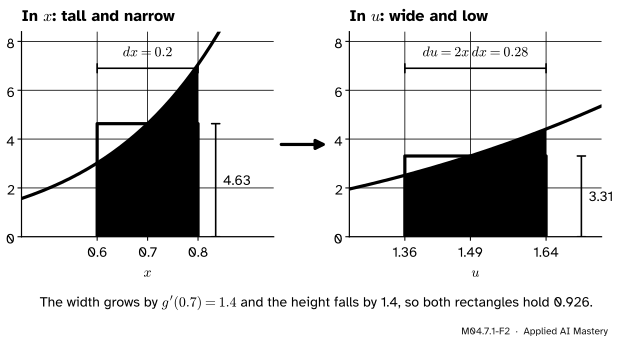
Step 4. Why \({du = g'(x)\,dx}\) is honest. Take the highlighted slice of the anchor figure and look at it closely.
M04.7.1-F2
One slice close up. In \(x\) the slice is 0.2 wide and about 4.63 tall; in \(u\) it is \({2 \times 0.7 \times 0.2 = 0.28}\) wide and about 3.31 tall. The width grows by \({g'(0.7) = 1.4}\) and the height falls by the same factor.
The slice from \({x = 0.6}\) to \({0.8}\) has width \({dx = 0.2}\). Its image runs from \({u = 1.36}\) to \({1.64}\), so \({du = 0.28}\), which is \({g'(0.7)\,dx = 1.4 \times 0.2}\). Over the slice, the height in \(x\) is \({f(g(x))\,g'(x)}\) and the height in \(u\) is \({f(u) = f(g(x))}\): one is the other times \({g'(x)}\). Height times width is the same in both. For a curved \(g\) the equation \({du = g'(x)\,dx}\) is only nearly true for a slice of finite width; it is the linear approximation of M04.2.2, and it becomes exact as the slices shrink, which is what an integral does.
The formal statement
NoteTheorem: the substitution rule
Let \(g\) have a continuous derivative on \({[a, b]}\), and let \(f\) be continuous on the values that \(g\) takes there. If \(F\) is an antiderivative of \(f\), then
\[
\int f\big(g(x)\big)\,g'(x)\,dx = F\big(g(x)\big) + C ,
\]
and for the definite integral the limits change with the variable:
so \({F(g(x))}\) is an antiderivative of the integrand on the left, which is the first statement. For the second, use part two of the fundamental theorem (M04.6.3) twice, once with each antiderivative:
Spot an inner function \(g(x)\) whose derivative multiplies the rest, perhaps up to a constant.
Write \({u = g(x)}\) and \({du = g'(x)\,dx}\), and rewrite the whole integrand in \(u\). No \(x\) may be left over.
Integrate in \(u\).
Put \({u = g(x)}\) back, or, for a definite integral, use the new limits \({g(a)}\) and \({g(b)}\). Then check by differentiating.
A constant factor is no obstacle. If the integrand has \(x\) where \({g'(x) = 2x}\), write \({x\,dx = du/2}\) and carry the \({1/2}\) along.
Go deeper: what if g turns back?
The proof never asked \(g\) to be increasing. Take \({\int_{-1}^{1} 2x\,(x^2 + 1)^3\,dx}\). Here \({u = x^2 + 1}\) starts at 2, falls to 1 at \({x = 0}\) and climbs back to 2, so the rule gives \({\int_2^2 u^3\,du = 0}\). The direct answer agrees, because the integrand is odd: the factor \({2x}\) changes sign while \({(x^2 + 1)^3}\) does not. So the area below the axis on the left cancels the area above it on the right. Where \(g\) decreases, \({du = g'(x)\,dx}\) is negative and the slices are traversed backwards, which is exactly how signed area (M04.5.3) keeps the books.
Worked example
Example 1: \({\int x\,e^{-x^2/2}\,dx}\). The inner function is \({u = x^2/2}\), and its derivative, \(x\), is the factor in front. So \({du = x\,dx}\) and
\[
\begin{aligned}
\int x\,e^{-x^2/2}\,dx &= \int e^{-u}\,du \\
&= -e^{-u} + C \\
&= -e^{-x^2/2} + C .
\end{aligned}
\]
The step \({\int e^{-u}\,du = -e^{-u} + C}\) is itself checked by differentiating: \({(-e^{-u})' = e^{-u}}\). And the whole answer is checked the same way:
The function \({x\,e^{-x^2/2}}\) is minus the slope of the bell curve \({e^{-x^2/2}}\), so its antiderivative had to be minus the bell curve. Remember the factor \(x\): lesson M04.7.4 is about the bell curve without it.
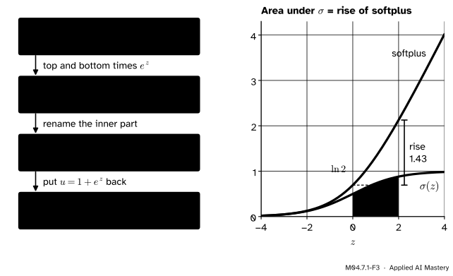
Example 2: the sigmoid. As written, \({1/(1 + e^{-z})}\) shows no inner function with its derivative beside it. Multiply top and bottom by \(e^z\) first:
Now the bottom, \({u = 1 + e^z}\), has derivative \(e^z\), which is the top. So \({du = e^z\,dz}\), and
\[
\begin{aligned}
\int \sigma(z)\,dz &= \int \frac{du}{u} = \ln u + C \\
&= \ln(1 + e^z) + C .
\end{aligned}
\]
No absolute value is needed, because \({u = 1 + e^z}\) is always positive. The antiderivative is softplus, which answers the question. From 0 to 2 the limits become \({u = 1 + e^0 = 2}\) and \({u = 1 + e^2 \approx 8.389}\):
The sigmoid by substitution, step by step (left), and what the answer means (right): the area under \(\sigma\) from 0 to 2 equals the rise of softplus over the same stretch, \({1.43}\).
Code
First, check each antiderivative the way this course always does: differentiate it numerically, with the central difference of M04.2.4, and compare the result with the integrand.
import mathdef central(F, x, h=1e-5):"""The slope of F at x by a central difference."""return (F(x + h) - F(x - h)) / (2* h)pairs = { # name: (integrand f, antiderivative F found by substitution)"2x(x^2+1)^3": (lambda x: 2* x * (x**2+1)**3, lambda x: (x**2+1)**4/4),"x e^(-x^2/2)": (lambda x: x * math.exp(-x**2/2), lambda x: -math.exp(-x**2/2)),"sigmoid": (lambda z: 1/ (1+ math.exp(-z)), lambda z: math.log(1+ math.exp(z))),}points = [-2, -1, -0.5, 0, 0.5, 1, 2]gaps = {}for name, (f, F) in pairs.items(): gaps[name] =max(abs(central(F, x) - f(x)) for x in points)print(f"{name:13s} max |F' - f| {gaps[name]:.1e}")
2x(x^2+1)^3   max |F' - f| 6.5e-08
x e^(-x^2/2)  max |F' - f| 2.1e-11
sigmoid       max |F' - f| 1.0e-11
Every gap is below \({10^{-7}}\), about the size of the central difference’s own error at this \(h\), so each \(F\) really is an antiderivative. Next, the two sides of the substitution rule, each computed from scratch with a midpoint sum, in \(x\) and in \(u\).
def midpoint_sum(f, a, b, n):"""The midpoint rule with n strips (M04.5.2).""" dx = (b - a) / nreturnsum(f(a + (k +0.5) * dx) for k inrange(n)) * dxin_x =lambda x: 2* x * (x**2+1)**3in_u =lambda u: u**3for n in (5, 50, 500):print(f"n = {n:3d}: in x {midpoint_sum(in_x, 0, 1, n):.6f} in u {midpoint_sum(in_u, 1, 2, n):.6f}")# The five slices of the anchor figure, exactly, from the antiderivatives in x and in u.xs = [0, 0.2, 0.4, 0.6, 0.8, 1.0]us = [x**2+1for x in xs]slice_x = [((b**2+1)**4- (a**2+1)**4) /4for a, b inzip(xs, xs[1:])]slice_u = [(d**4- c**4) /4for c, d inzip(us, us[1:])]print("u cuts: ", [round(u, 2) for u in us])print("slices in x: ", [round(s, 4) for s in slice_x])print("slices in u: ", [round(s, 4) for s in slice_u])
n =   5:  in x 3.648173   in u 3.735000
n =  50:  in x 3.748967   in u 3.749850
n = 500:  in x 3.749990   in u 3.749999
u cuts:       [1, 1.04, 1.16, 1.36, 1.64, 2.0]
slices in x:  [0.0425, 0.1602, 0.4026, 0.9532, 2.1915]
slices in u:  [0.0425, 0.1602, 0.4026, 0.9532, 2.1915]
Both midpoint sums close in on \({15/4 = 3.75}\), and the slices match pair by pair, as the anchor figure showed. Now the library: scipy.integrate.quad computes each definite integral and reports an estimate of its own error.
import numpy as npfrom scipy import integratecases = [ ("2x(x^2+1)^3 on [0, 1]", in_x, 0, 1, 15/4), ("x e^(-x^2/2) on [0, 2]", lambda x: x * np.exp(-x**2/2), 0, 2, 1- math.exp(-2)), ("sigmoid on [0, 2]", lambda z: 1/ (1+ np.exp(-z)), 0, 2, math.log((1+ math.e**2) /2)),]for name, f, a, b, by_hand in cases: value, error = integrate.quad(f, a, b)print(f"{name:24s} quad {value:.6f} (error estimate {error:.0e}) by hand {by_hand:.6f}")print("softplus(1000) with logaddexp:", np.logaddexp(0, 1000.0))
2x(x^2+1)^3 on [0, 1]    quad 3.750000  (error estimate 4e-14)   by hand 3.750000
x e^(-x^2/2) on [0, 2]   quad 0.864665  (error estimate 1e-14)   by hand 0.864665
sigmoid on [0, 2]        quad 1.433781  (error estimate 2e-14)   by hand 1.433781
softplus(1000) with logaddexp: 1000.0
The last line is a practical point. Written as math.log(1 + math.exp(z)), softplus overflows for large \(z\), because \({e^{1000}}\) is far beyond the largest floating-point number. np.logaddexp(0, z) computes \({\ln(e^0 + e^z)}\) without ever forming \(e^z\), which is how machine-learning libraries evaluate softplus.
Explore
M04.7-X1
Substitution viewer
Pick an integral, then drag the limits \(a\) and \(b\) on the top graph, or use the sliders. The bottom graph shows the same integral after the substitution: its limits \({g(a)}\) and \({g(b)}\) and its slices move with yours, and the read-out compares the two areas and the highlighted slice.
Things to try:
With \({2x(x^2 + 1)^3}\), step the highlighted slice from the first to the last. Near \({x = 0}\) the \(u\)-slice is squeezed, because \({g'(x) = 2x}\) is small; the last one is almost twice as wide as in \(x\).
Drag \(b\) down to 0.5. The \(u\)-limit \({g(b) = b^2 + 1}\) follows it to 1.25, and both areas shrink together to \({(1.25^4 - 1)/4 \approx 0.3604}\).
With \({x\,e^{-x^2/2}}\), push \(b\) to its largest value, \({b = 2}\). The area is \({1 - e^{-2} \approx 0.865}\) in both panels; lesson M04.7.3 lets \(b\) run on to infinity.
With the sigmoid, compare the first and the last slice: \({du = e^z\,dz}\), so the first is squeezed to about a fifth of its width in \(u\) and the last is stretched more than three times, while each pair of slices still holds equal areas.
Pitfalls
M04.7.1-F4
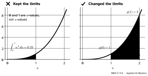
Wrong beside right. After the substitution \({u = x^2 + 1}\), keeping the old limits 0 and 1 measures the wrong region (left, 0.25). The limits must move to \({g(0) = 1}\) and \({g(1) = 2}\) (right, 3.75).
“Substitute, integrate, then use the original limits.”
After the substitution the integrand is a function of \(u\), and 0 and 1 are values of \(x\). Either change the limits to \({g(a)}\) and \({g(b)}\), or put \({u = g(x)}\) back before you use \(a\) and \(b\). Mixing the two gives \({\int_0^1 u^3\,du = 0.25}\) instead of \({15/4}\).
“Any inner function will do; divide by its derivative if it is missing.”
\({\int (x^2 + 1)^3\,dx}\) has the same inner function but no factor \({2x}\). Writing \({dx = du/(2x)}\) leaves an \(x\) inside a \(u\)-integral, which is not allowed: \(x\) is not a constant. Only constant factors can be moved outside. This integral is still easy (expand the cube), but \({\int e^{-x^2/2}\,dx}\) is not: no substitution works, and lesson M04.7.4 shows what to do instead.
“The \(dx\) is decoration, so I can drop it.”
The \(dx\) is where the stretch factor lives. Turning \({e^{-x^2/2}\,x\,dx}\) into \({e^{-u}\,du}\) is legal only because \({x\,dx}\) is exactly \(du\). A substitution that forgets the \(dx\) changes the area, and differentiating the answer will expose it. In machine learning the same bookkeeping keeps a probability density honest when a variable is rescaled: see the box below.
Frontier note: the reparameterisation trick is a substitution
A variational autoencoder must differentiate an average, the integral of \({p(z)\,f(z)}\) over \(z\), where \(p\) is a normal density with mean \(\mu\) and scale \(s\) that the network is learning. Kingma and Welling (Section 2.4) substitute \({z = \mu + s\,\varepsilon}\), where \(\varepsilon\) has the standard normal density. Then \({dz = s\,d\varepsilon}\) and the density keeps its probability slice by slice, \({p(z)\,dz = p(\varepsilon)\,d\varepsilon}\), so the average becomes the integral of \({p(\varepsilon)\,f(\mu + s\,\varepsilon)}\) over \(\varepsilon\). Now \(\mu\) and \(s\) sit inside \(f\), where the chain rule can reach them, and the average can be estimated from samples of \(\varepsilon\). It is the \({du = g'(x)\,dx}\) of this lesson, with \({g(\varepsilon) = \mu + s\,\varepsilon}\) and \({g' = s}\).
Check yourself
Recall
1. Which rule of differentiation does substitution undo, and how?
Show answer
The chain rule. Since \({(F(g(x)))' = f(g(x))\,g'(x)}\) when \({F' = f}\), the function \({F(g(x))}\) is an antiderivative of \({f(g(x))\,g'(x)}\).
2. In \({\int 2x\,(x^2 + 1)^3\,dx}\), what are \(u\) and \(du\), and what is the antiderivative?
Show answer
\({u = x^2 + 1}\) and \({du = 2x\,dx}\), so the integral is \({\int u^3\,du = u^4/4 + C}\), that is, \({(x^2 + 1)^4/4 + C}\).
3. When you substitute \({u = g(x)}\) in an integral from \(a\) to \(b\), what are the new limits?
Show answer
\({g(a)}\) and \({g(b)}\): the values of the new variable at the old ends.
4. What is an antiderivative of the sigmoid, and which substitution finds it?
Show answer
Softplus, \({\ln(1 + e^z)}\). Write \({\sigma(z) = e^z/(1 + e^z)}\) and substitute \({u = 1 + e^z}\), so \({du = e^z\,dz}\) and the integral becomes \({\int du/u = \ln u + C}\).
5. How do you check an antiderivative found by substitution?
Show answer
Differentiate it, by hand or with a central difference at a few points, and compare the result with the integrand.
Exercises
1.★ Find \({\int 3x^2\,(x^3 + 1)^4\,dx}\) and then \({\int_0^1 3x^2\,(x^3 + 1)^4\,dx}\).
Show solution
The inner function is \({u = x^3 + 1}\), and \({du = 3x^2\,dx}\) is the factor in front. So the integral is \({\int u^4\,du = u^5/5 + C}\), that is, \({(x^3 + 1)^5/5 + C}\). For the definite integral the limits become \({u = 1}\) and \({u = 2}\):
3.★★★ Show that \({\int_{-a}^{a} \sigma(z)\,dz = a}\) for every \({a > 0}\), in two ways: with softplus, and with the substitution \({z = -w}\) on the left half together with \({\sigma(w) + \sigma(-w) = 1}\).
Show solution
With softplus. The integral is \({\ln(1 + e^a) - \ln(1 + e^{-a})}\). Multiply the inside of the second logarithm by \({e^a/e^a}\): \({1 + e^{-a} = (e^a + 1)/e^a}\), so
so the integral is \({\int_0^a 1\,dw = a}\). For \({a = 2}\) the area is exactly 2.
Summary card
Substitution is the chain rule run backwards: rename the inner function, and its derivative pays for the change.
M04.7.1-F1
Same area, stretched slices.
The rule. If \({F' = f}\), then \({F(g(x))}\) is an antiderivative of \({f(g(x))\,g'(x)}\).
Definite form. The limits change from \(a\) and \(b\) to \({g(a)}\) and \({g(b)}\).
The bookkeeping.\({du = g'(x)\,dx}\): width times \({g'}\), height divided by \({g'}\).
Two results.\({x\,e^{-x^2/2}}\) integrates to \({-e^{-x^2/2}}\), and \(\sigma\) to softplus, \({\ln(1 + e^z)}\).
Sources and next steps
Sources. Each was opened and checked against this lesson on 12 November 2026.
Gilbert Strang and Edwin Herman, Calculus Volume 2 (OpenStax), Section 1.5, Substitution: Theorem 1.7 (substitution with indefinite integrals), Theorem 1.8 (substitution with definite integrals, where the limits become \({g(a)}\) and \({g(b)}\)), its problem-solving strategy, and Example 1.30, a polynomial of the same shape as ours.
Matthew Boelkins, Active Calculus (single variable), Section 5.3, Integration by substitution: substitution as reversing the chain rule (Subsection 5.3.3) and the warning that a substitution in a definite integral also changes its limits (Subsection 5.3.4).
David Jerison, MIT OpenCourseWare 18.01SC, Session 38, Integration by substitution: the notes of the clip More examples of integration find \({\int x\,e^{-x^2}\,dx = -\tfrac12 e^{-x^2} + c}\) and warn that an answer not checked by differentiating is likely to be wrong.
Diederik Kingma and Max Welling, Auto-Encoding Variational Bayes, Section 2.4: the reparameterisation \({z = \mu + \sigma\varepsilon}\) and the identity that turns an integral over \(z\) into one over \(\varepsilon\) (they write \(\sigma\) for the scale that this lesson calls \(s\)).
Next.M04.7.2 Integration by parts runs the product rule backwards, for integrals such as \({\int x\,e^x\,dx}\) where no inner function’s derivative appears.