Area below the axis counts as negative, so an integral is a net amount: a velocity integrates to net distance, not distance travelled. Derive linearity, splitting, reversing and comparison from the sums, then use them for the average value of a function and a first probability.
Explain why area below the horizontal axis counts as negative in an integral, and tell net distance from distance travelled.
Derive linearity, splitting an interval, reversing the limits and comparison from the Riemann sums, and use them to integrate simple polynomials.
Compute the average value of a function as its integral divided by the length of the interval, and explain it as the limit of an ordinary mean of samples.
Find a probability as an area under a density, after checking that the total area is 1.
In review. The maths and code on this page are checked by automated tests on every change, but an independent reader has not signed it off yet. Spot a mistake or a confusing step? Tell us.
The question
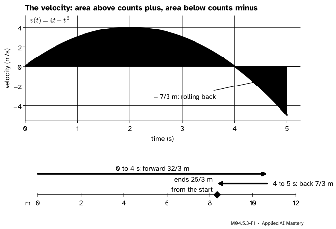
Let the cart’s motor run for a fifth second. After \({t = 4}\) its velocity, \({v(t) = 4t - t^2}\), turns negative and the cart rolls backwards. Where is it at \({t = 5}\), and how far has it travelled? The two answers differ, and the integral of the velocity gives only the first. An integral taken of a probability density gives a probability, and divided by the length of the interval it gives an average: the continuous version of the mean that machine learning computes all day.
From the last lesson
1. What is \({\int_0^1 x^2\,dx}\), and why is no right sum with finitely many strips exactly equal to it?
Show answer
1/3. It is the limit of the right sums, and each one is off: the right sum with \(n\) strips is \({1/3 + 1/(2n) + 1/(6n^2)}\), which is above 1/3 for every \(n\).
2. Name the integrand and the limits of integration in \({\int_a^b f(x)\,dx}\).
Show answer
The integrand is \({f(x)}\), and the limits of integration are \(a\) and \(b\).
Intuition
A Riemann sum adds terms \({f(x_k^*)\,\Delta x}\), and nothing forces the heights to be positive. Where the graph dips below the axis the height is negative, so the term is minus the rectangle’s area. Area above the axis adds, and area below the axis subtracts.
M04.5.3-F1
The integral of a velocity is a net amount. The area above the axis is distance forward; the hatched area below it is distance back and counts with a minus sign. The cart ends 25/3 m from where it started.
For a velocity this is exactly right. The integral from 0 to 5 adds the forward distance and takes away the backward distance, so it gives the change in position, the net distance, often called the displacement. The distance the wheels actually rolled, the distance travelled, counts every part as positive.
Build it up
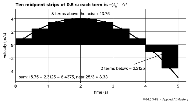
Step 1. The sign of a term. The strip width \({\Delta x = (b - a)/n}\) is positive when \({a < b}\). So the term \({f(x_k^*)\,\Delta x}\) has the sign of the height: positive above the axis, negative below it.
M04.5.3-F2
A Riemann sum with ten midpoint rectangles. The two rectangles that hang below the axis have negative heights, so their terms subtract.
Step 2. Net signed area. In the limit, the integral is the area above the axis minus the area below it:
This is the net signed area. For the cart, \({A_{\text{above}} = 32/3}\) and \({A_{\text{below}} = 7/3}\) (the worked example finds both), so the integral is 25/3.
Step 3. Total area. To count every part as positive, integrate the size of the function, \({\abs{f(x)}}\), which flips the parts below the axis up above it. For a velocity, \({\abs{v}}\) is the speed, and its integral is the distance travelled: \({32/3 + 7/3 = 13}\) m.
Step 4. Rules. Splitting the trip at \({t = 4}\), flipping a sign, combining \(t\) and \({t^2}\) into \({4t - t^2}\): these need rules for integrals. Each one comes straight from a rule for sums.
The formal statement
Three integrals we already know. A constant \(c\) gives every Riemann sum the value \({c\,(b - a)}\), so \({\int_a^b c\,dx = c\,(b - a)}\). The region under \({y = x}\) from 0 to \(b\) is a triangle, so \({\int_0^b x\,dx = b^2/2}\). And lesson M04.5.2 found \({\int_0^b x^2\,dx = b^3/3}\).
Below, \(f\) and \(g\) are continuous on \({[a, b]}\), so every integral exists, and the sums use the same strips and sample points for both functions.
Rule 1: linearity. For numbers \(c\) and \(d\),
\[
\begin{aligned}
&\int_a^b \big(c\,f(x) + d\,g(x)\big)\,dx \\
&\quad = c \int_a^b f(x)\,dx + d \int_a^b g(x)\,dx .
\end{aligned}
\]
Why. Each Riemann sum splits the same way, by the sigma rules of M01.7.2 (a constant factor comes out, a sum of sums splits):
\[
\begin{aligned}
&\sum \big(c\,f(x_k^*) + d\,g(x_k^*)\big)\,\Delta x \\
&\quad = c \sum f(x_k^*)\,\Delta x \\
&\qquad + d \sum g(x_k^*)\,\Delta x .
\end{aligned}
\]
Now let \(n\) grow. The limit of a sum is the sum of the limits, and a constant factor comes out of a limit (M04.1.2), so the integrals split in the same way.
Rule 2: splitting the interval. For a point \(c\) between \(a\) and \(b\),
Why. Choose \(n\) so that \(c\) falls on a cut point; for \({c = 4}\) in \({[0, 5]}\) any multiple of 5 will do. Then the strips to the left of \(c\) cut \({[a, c]}\) into equal strips, the strips to the right cut \({[c, b]}\), and the sigma splits into the sum over the first group plus the sum over the second. As \(n\) grows, each part tends to its own integral. (Such an \(n\) exists whenever \(c\) cuts the interval in a ratio of whole numbers. The rule holds for every \(c\), but the proof for the other points needs a finer argument from analysis, which this course leaves out.)
Rule 3: reversing the limits. Run a sum from \(b\) back to \(a\): the strip width is \({(a - b)/n}\), which is negative, so every term changes sign. That gives
\[
\int_b^a f(x)\,dx = -\int_a^b f(x)\,dx ,
\]
and with \({a = b}\) the width is 0, so \({\int_a^a f(x)\,dx = 0}\). With these two conventions, Rule 2 holds whatever the order of \(a\), \(b\) and \(c\).
Rule 4: comparison. If \({f(x) \le g(x)}\) for every \(x\) in \({[a, b]}\), with \({a < b}\), then
\[
\int_a^b f(x)\,dx \le \int_a^b g(x)\,dx .
\]
Why. Each term obeys \({f(x_k^*)\,\Delta x \le g(x_k^*)\,\Delta x}\), because \({\Delta x > 0}\). So every sum for \(f\) is at most the matching sum for \(g\), and the inequality survives the limit. Taking \(f\) or \(g\) constant gives a quick bound: if \({m \le f(x) \le M}\) on \({[a, b]}\), then
\[
\begin{aligned}
m\,(b - a) &\le \int_a^b f(x)\,dx \\
&\le M\,(b - a) .
\end{aligned}
\]
Go deeper: why an inequality survives the limit
Suppose \({p_n \le q_n}\) for every \(n\), with \({p_n \to p}\) and \({q_n \to q}\). The differences \({q_n - p_n}\) are never negative and tend to \({q - p}\). If \({q - p}\) were negative, say \({-\varepsilon}\), then from some \(n\) on every difference would lie within \({\varepsilon/2}\) of \({-\varepsilon}\), and so would be negative, which is impossible. So \({q - p \ge 0}\). The same argument does not give strict inequality: \({0 < 1/n}\) for every \(n\), but both sides tend to 0.
The average value. Sample \(f\) at the sample points of \(n\) equal strips and take the ordinary mean of the \(n\) values. Since \({\Delta x = (b - a)/n}\), we have \({1/n = \Delta x/(b - a)}\), so
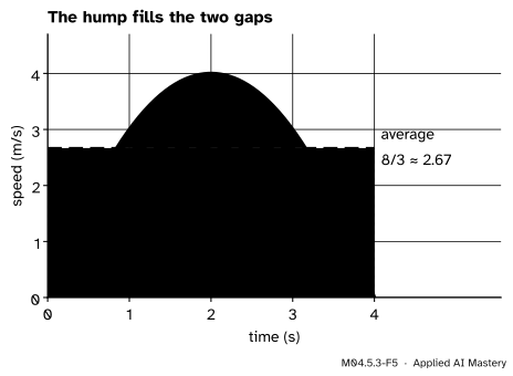
The average value is the height of the rectangle with the same width and the same area as the region under the curve. The hump above the dashed line exactly fills the two gaps below it.
By Rule 4 with \({m = \min f}\) and \({M = \max f}\), dividing by \({b - a}\) shows that the average value always lies between the smallest and the largest value of \(f\).
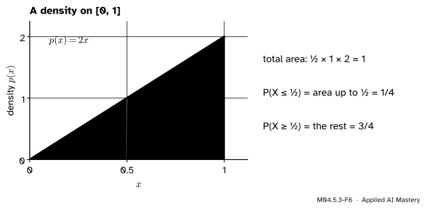
A first look at probability. A probability density on an interval is a function \({p(x) \ge 0}\) whose total area is 1. A random number \(X\) with that density lands between \(a\) and \(b\) with probability equal to the area there:
\[
\Prob(a \le X \le b) = \int_a^b p(x)\,dx .
\]
M04.5.3-F6
The density \({p(x) = 2x}\) on \({[0, 1]}\): the total area is 1, and the probability of landing below one half is the area up to one half, 1/4.
For \({p(x) = 2x}\) on \({[0, 1]}\), linearity and the triangle give a total of \({2 \times 1/2 = 1}\), and \({\Prob(X \le 1/2) = 2 \times (1/2)^2/2 = 1/4}\). Module M06.6 builds continuous probability on this.
Worked example
The cart runs on to \({t = 5}\). Find its net distance, its distance travelled, its average velocity and its average speed.
The integral from 0 to \(b\). By linearity, then the triangle and the square,
This is the position formula \({s(b)}\) of the cart, as it should be. At \({b = 4}\) it gives \({32 - 64/3 = 32/3}\), and at \({b = 5}\) it gives \({50 - 125/3 = 25/3}\).
Split at \({t = 4}\), where the velocity changes sign. By Rule 2,
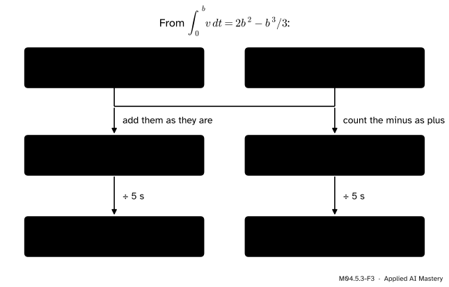
The worked example as a trace. Both pieces feed both answers: added as they are they give the net distance, and with the minus counted as plus they give the distance travelled.
Net distance.\({32/3 - 7/3 = 25/3 \approx 8.33}\) m: the cart ends 8.33 m from its start.
Distance travelled. The speed \({\abs{v}}\) equals \(v\) up to \({t = 4}\) and \({-v}\) after it, so by Rules 2 and 1
Averages. Dividing by the 5 seconds, the average velocity is \({(25/3)/5 = 5/3 \approx 1.67}\) m/s and the average speed is \({13/5 = 2.6}\) m/s. Over the first 4 seconds alone the average speed is \({(32/3)/4 = 8/3 \approx 2.67}\) m/s, the dashed line in the average-value figure.
Code
A midpoint sum with many strips stands in for each integral. It checks the worked example, the rules and the average, all in a few lines.
import numpy as npdef integral(f, a, b, n=100_000):"""A midpoint sum with n strips; the width is negative when b < a.""" dx = (b - a) / n x = a + (np.arange(n) +0.5) * dxreturn np.sum(f(x)) * dxdef v(t):return4* t - t **2print("net distance, 0 to 5 s: ", round(integral(v, 0, 5), 4))print("distance travelled: ", round(integral(lambda t: np.abs(v(t)), 0, 5), 4))print("the backward part, 4 to 5:", round(integral(v, 4, 5), 4))print("limits reversed, 5 to 4: ", round(integral(v, 5, 4), 4))
net distance, 0 to 5 s:    8.3333
distance travelled:         13.0
the backward part, 4 to 5: -2.3333
limits reversed, 5 to 4:    2.3333
The numbers match the worked example: 8.3333, 13.0, \({-2.3333}\), and 2.3333 with the limits reversed. Next, linearity, comparison and the average value, which is just numpy.mean of many evenly spread samples.
f, g = (lambda x: x), (lambda x: x **2)lhs = integral(lambda x: 4* f(x) - g(x), 0, 4)rhs =4* integral(f, 0, 4) - integral(g, 0, 4)print("linearity:", round(lhs, 6), "=", round(rhs, 6))print("comparison on [0, 1], x^2 <= x:", round(integral(g, 0, 1), 4), "<=", round(integral(f, 0, 1), 4))samples = v(np.linspace(0, 4, 1_000_001)) # a million and one evenly spread speedsprint("mean of the samples:", round(np.mean(samples), 4), " 8/3 =", round(8/3, 4))p =lambda x: 2* x # the density of the formal sectionprint("total probability:", round(integral(p, 0, 1), 6), " P(X <= 1/2):", round(integral(p, 0, 0.5), 6))
linearity: 10.666667 = 10.666667
comparison on [0, 1], x^2 <= x: 0.3333 <= 0.5
mean of the samples: 2.6667   8/3 = 2.6667
total probability: 1.0   P(X <= 1/2): 0.25
The mean of a million evenly spread speeds is 2.6667 to four places, the average value 8/3. In machine learning the same idea runs the other way: an expected value is an integral, and it is estimated by the mean of many samples.
Explore
This module’s interactive, the Riemann refiner, lives in lesson M04.5.2. Choose Cart run on to 5 s: the strips after \({t = 4}\) hang below the axis, and every rule closes in on the net value 25/3, not on the distance travelled.
Pitfalls
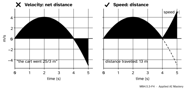
M04.5.3-F4
Wrong beside right. Integrating the velocity gives the net distance, 25/3 m. The distance travelled integrates the speed \({\abs{v}}\), 13 m.
“The integral of the velocity is the distance travelled.”
It is the net distance: the backward part counts against the forward part. The cart rolled 13 m in all but ended only 25/3 m from its start. For the distance travelled, integrate \({\abs{v}}\), which in practice means splitting at each zero of \(v\) and adding the sizes of the pieces.
“An integral is an area, so it is never negative.”
An integral is a signed area. \({\int_4^5 v\,dt = -7/3}\), and \({\int_{-1}^{1} x\,dx = 0}\), because the triangle below the axis cancels the one above. Even a positive function gives a negative integral when the limits run backwards: \({\int_1^0 x^2\,dx = -1/3}\).
“The average value is the average of the two end values.”
For the speed on \({[0, 4]}\), the end values are 0 and 0, and the smallest and largest values are 0 and 4, so those shortcuts give 0 or 2. The average value is \({(32/3)/4 = 8/3}\). A function’s average weighs every point of the interval, as a mean weighs every data point.
Check yourself
Recall
1. Why does area below the axis count as negative in an integral?
Show answer
Below the axis the heights \({f(x_k^*)}\) are negative while the widths \({\Delta x}\) are positive, so those terms of every Riemann sum, and so of the limit, are negative.
2. For a velocity \(v\), what do \({\int_a^b v\,dt}\) and \({\int_a^b \abs{v}\,dt}\) measure?
Show answer
The first is the net distance, the change in position. The second is the distance travelled.
3. State the splitting rule and the rule for reversed limits.
Show answer
\({\int_a^b f = \int_a^c f + \int_c^b f}\), and \({\int_b^a f = -\int_a^b f}\), with \({\int_a^a f = 0}\).
4. What does linearity say?
Show answer
For any numbers \(c\) and \(d\),
\[
\begin{aligned}
&\int_a^b (c\,f + d\,g)\,dx \\
&\quad = c \int_a^b f\,dx + d \int_a^b g\,dx .
\end{aligned}
\]
5. Give the formula for the average value of \(f\) on \({[a, b]}\), and the cart’s average speed over its first 4 seconds.
Show answer
\({f_{\text{avg}} = \frac{1}{b - a} \int_a^b f(x)\,dx}\). For the cart, \({(32/3)/4 = 8/3 \approx 2.67}\) m/s.
Exercises
1.★ Find \({\int_0^3 (2x + 1)\,dx}\) with linearity, then check it with the area of a trapezoid.
The region is a trapezoid with parallel sides \({f(0) = 1}\) and \({f(3) = 7}\) and width 3, so its area is \({3 \times (1 + 7)/2 = 12}\). They agree.
2.★★ The running cubic \({g(x) = x^3 - 3x}\) has \({g(-x) = -g(x)}\). Explain with midpoint sums why \({\int_{-2}^{2} g(x)\,dx = 0}\). Is the area between the curve and the axis 0?
Show solution
With \(n\) equal strips on \({[-2, 2]}\), the midpoints come in pairs \(x\) and \({-x}\), one on each side of 0 (with 0 itself as the middle midpoint when \(n\) is odd, where \({g(0) = 0}\)). In each pair the heights are \({g(x)}\) and \({-g(x)}\), which cancel. So every midpoint sum is exactly 0, and so is their limit. The area between the curve and the axis is not 0. Because \({g(-x) = -g(x)}\), the region over \({[-2, 0]}\) is the region over \({[0, 2]}\) mirrored and flipped to the other side of the axis: each piece above the axis on one side has a twin of the same size below it on the other. The integral counts the twins with opposite signs, so they cancel, while the area counts both as positive. The total area is twice the area between the curve and the axis on \({[0, 2]}\).
3.★★★ The sigmoid is \({\sigma(z) = 1/(1 + e^{-z})}\). Show that \({\sigma(-z) = 1 - \sigma(z)}\), then show that every midpoint sum of \(\sigma\) on \({[-4, 4]}\) equals 4. What are \({\int_{-4}^{4} \sigma(z)\,dz}\) and the average value of \(\sigma\) on that interval?
Show solution
Multiply the top and bottom of \({\sigma(-z) = 1/(1 + e^{z})}\) by \({e^{-z}}\):
With \(n\) strips of width \({8/n}\), the midpoints pair up as \(z\) and \({-z}\), and each pair’s heights add to \({\sigma(z) + \sigma(-z) = 1}\); for odd \(n\) the middle midpoint is 0, with \({\sigma(0) = 1/2}\). Either way the \(n\) heights add to \({n/2}\), so the midpoint sum is \({(8/n)(n/2) = 4}\) for every \(n\). Its limit is 4, so \({\int_{-4}^{4} \sigma(z)\,dz = 4}\) and the average value is \({4/8 = 1/2}\).
Summary card
An integral is a net amount: area above the axis adds, area below subtracts.
M04.5.3-F1
Forward 32/3, back 7/3, net 25/3.
Net and total.\({\int v\,dt}\) is the net distance; \({\int \abs{v}\,dt}\) is the distance travelled.
Linearity. Constants come out, and the integral of a sum is the sum of the integrals.
Splitting and reversing.\({\int_a^b f = \int_a^c f + \int_c^b f}\), and \({\int_b^a f = -\int_a^b f}\).
Comparison. If \({f \le g}\) on \({[a, b]}\), then \({\int_a^b f \le \int_a^b g}\).
Average value.\({f_{\text{avg}} = \frac{1}{b - a} \int_a^b f(x)\,dx}\).
Sources and next steps
Sources. Each was opened and checked against this lesson on 12 November 2026.
Gilbert Strang and Edwin Herman, Calculus Volume 1 (OpenStax), Section 5.2, The Definite Integral. It defines net signed area and total area, shows a car whose northward and southward trips give zero displacement but a positive total distance, lists the properties of the definite integral (equations 5.9 to 5.14), states the comparison theorem (Theorem 5.2) and defines the average value of a function.
Matthew Boelkins, Active Calculus, Section 4.1, where negative area distinguishes distance travelled from change in position, and Section 4.3, which derives the average value from the average of \(n\) sampled values and draws the rectangle with the same area.
Barbara Illowsky and Susan Dean, Introductory Statistics 2e (OpenStax), Section 5.1, Continuous Probability Functions, for continuous probability as area under a density curve, with a maximum area of one.