Two inputs, one output: surfaces and contour lines
A function of two inputs gives a height at every point of the plane. Draw it as a surface or, from above, as contour lines like a hiking map, cut slices through it by freezing one input, and read a loss with two parameters the same way.
Evaluate a function of two inputs and build a table of its heights on a grid.
Find and draw the contour lines of a function, and read their spacing as steepness.
Cut a slice by freezing one input, and write it as a function of the other input.
Compute the mean squared error of a line as a function of its slope and intercept, and find its lowest value on a grid with NumPy.
In review. The maths and code on this page are checked by automated tests on every change, but an independent reader has not signed it off yet. Spot a mistake or a confusing step? Tell us.
The question
A model with one weight has a loss you can draw as a curve and walk down to its lowest point (M04.4). The line \({\hat{y} = wx + b}\) has two numbers to tune, the slope \(w\) and the intercept \(b\), so its loss depends on two inputs at once, and a graph with one input axis has no room for that. How do you draw a function of two inputs, and how do you see where it is lowest? Map makers solved the same problem for mountains long ago.
Intuition
Think of the plane of inputs as the ground and the output as a height. A function of two inputs takes a point \((x, y)\) of the plane and gives one number, \(f(x, y)\). Stand a pole of that height at every point, and the tops of the poles form a surface: a landscape over the plane.
This module’s first example is the running bowl, \({f(x, y) = x^2 + 2y^2}\). It is 0 at the origin and grows in every direction, faster along \(y\) than along \(x\), because \(y\) is squared and then doubled.
M04.10.1-F1
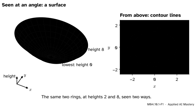
The running bowl \({f(x, y) = x^2 + 2y^2}\) two ways. Seen at an angle it is a surface. Seen from above, each height becomes a ring, a contour line, and the lowest point is the star.
From above, the surface becomes a set of contour lines, each joining the points of one height, like the lines on a hiking map. The right panel shows three things without any algebra. The lowest point is the centre. Every ring is an oval, longer along \(x\) than along \(y\). And the ring at height 8 reaches \({x = 2.83}\) but only \({y = 2}\), so the climb to height 8 is shorter, and steeper, along \(y\).
Build it up
Step 1. Two numbers in, one number out. To evaluate \(f\), put in both numbers: \({f(1, 1)} = {1 + 2} = {3}\) and \({f(2, -1)} = {4 + 2} = {6}\). The order matters: \({f(2, 1) = 6}\) but \({f(1, 2) = 9}\), because the second input is the one that gets doubled.
Step 2. A table of heights. Evaluate \(f\) at every point of a grid and write each height at its point. That is a map with numbers on it, the raw material of every contour map. The worked example below builds one for 25 points.
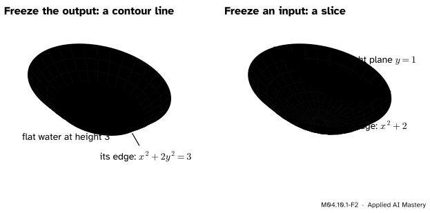
Step 3. Contour lines: freeze the output. Choose a height \(c\) and mark every point where \({f(x, y) = c}\). Picture filling the bowl with water up to height 3. The water’s flat surface is a level plane, and its edge, where water meets bowl, is the contour line at height 3.
Step 4. Slices: freeze an input. Now hold \(y\) fixed, say at \({y = 1}\), and let only \(x\) move. What is left is an ordinary function of one variable, \({f(x, 1) = x^2 + 2}\), a parabola. On the surface it is the curve cut out by an upright plane, the way a knife cuts a cake.
M04.10.1-F2
Two ways to cut the bowl. A level cut at height 3 leaves the oval \({x^2 + 2y^2 = 3}\); an upright cut at \({y = 1}\) leaves the parabola \({x^2 + 2}\).
A contour line lives in the plane of the inputs and has one height all along it. A slice is an ordinary graph of height against one input. This module uses contour lines to see the landscape and slices to measure its slopes.
The formal statement
NoteDefinitions: functions of two variables, contour lines and slices
A function of two variables\(f\) assigns to each point \((x, y)\) of a set \(D\) in the plane exactly one number, \(f(x, y)\). Its graph is the surface of points \({(x, y, z)}\) with \({z = f(x, y)}\).
The contour line (or level curve) of \(f\) at height \(c\) is the set of points \((x, y)\) where \({f(x, y) = c}\). A picture of several contour lines is a contour map.
The slice of \(f\) through \({y = y_0}\) is the function of one variable \({x \mapsto f(x, y_0)}\). The slice through \({x = x_0}\) is \({y \mapsto f(x_0, y)}\).
A contour line is a set of points in the plane; a slice is a function. Two contour lines at different heights never cross, because a point where they met would have two heights, and a function gives each point exactly one.
The contour lines of the bowl. Set \({x^2 + 2y^2 = c}\) for a height \({c > 0}\). On the \(x\) axis, where \({y = 0}\), this leaves \({x^2 = c}\), so the line crosses the axis at \({x = \pm\sqrt{c}}\). On the \(y\) axis it leaves \({2y^2 = c}\), so \({y = \pm\sqrt{c/2}}\). Dividing the equation by \(c\) shows the shape:
\[
\frac{x^2}{c} + \frac{y^2}{c/2} = 1 .
\]
Write \({u = x/\sqrt{c}}\) and \({v = y/\sqrt{c/2}}\). Then \({u^2 + v^2 = 1}\), the unit circle. So each contour line is a circle stretched by \(\sqrt{c}\) along \(x\) and by \(\sqrt{c/2}\) along \(y\): an ellipse. The ratio of its two half-widths is the same for every height,
so every ring has the same oval shape, only bigger. At \({c = 0}\) the ring shrinks to the single point \((0, 0)\), and for \({c < 0}\) there is no ring at all, because a sum of squares is never negative.
Spacing shows steepness. From height 2 to height 8 the rings move out along \(x\) from \({\sqrt{2} \approx 1.41}\) to \({\sqrt{8} \approx 2.83}\), a walk of 1.41, but along \(y\) only from 1 to 2, a walk of 1. The same climb over a shorter walk means steeper ground. In general, where contour lines at equal steps of height crowd together, the function changes fast; where they spread out, it is nearly flat.
Go deeper: why every slice of the bowl is a parabola
Freeze \({y = y_0}\): the slice is \({x^2 + 2y_0^2}\), the parabola \(x^2\) lifted by the constant \({2y_0^2}\). Freeze \({x = x_0}\): the slice is \({2y^2 + x_0^2}\), the narrower parabola \(2y^2\) lifted by \(x_0^2\). Only the lift changes from slice to slice. The narrower parabolas are the steeper ground along \(y\) seen in profile; lesson 2 measures how much steeper.
Worked example
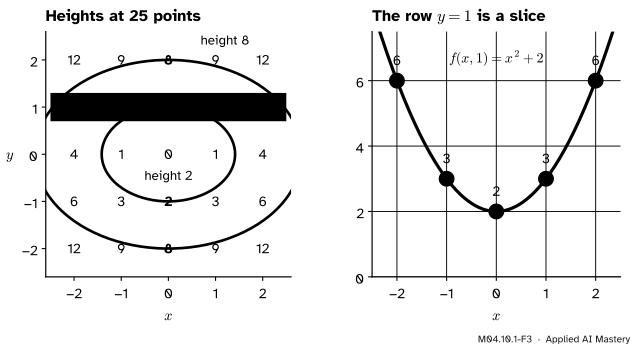
The running bowl by hand. Take the 25 points whose coordinates \(x\) and \(y\) are each one of \({-2, -1, 0, 1, 2}\). The row \({y = 1}\) reads \({f(-2, 1)} = {4 + 2} = {6}\), then 3, 2, 3 and 6. The row \({y = 2}\) reads 12, 9, 8, 9, 12, because \({2 \times 2^2 = 8}\) is added to each square. The rows \({y = -1}\) and \({y = -2}\) repeat the rows for 1 and 2, because \(y\) is squared.
M04.10.1-F3
The worked example as a trace. The table of heights with the contour lines at 2 and 8 threaded through it (left), and its row \({y = 1}\) read as the slice \({x^2 + 2}\) (right).
Two contour lines can be drawn through the table. Height 2 is reached at \({(0, \pm 1)}\) and, between grid points, at \({(\pm\sqrt{2}, 0)}\): the ellipse with half-widths 1.41 and 1. Height 8 is reached at \({(0, \pm 2)}\), and also at \({(\pm 2, \pm\sqrt{2})}\) since \({4 + 2 \times 2 = 8}\): the ellipse with half-widths 2.83 and 2. Every number inside the ring at 2 is below 2, and every number outside it is above. The row \({y = 1}\), read on its own, is the slice \({x^2 + 2}\): lowest, 2, at \({x = 0}\), and climbing to 6 at \({x = \pm 2}\).
A loss with two inputs. The running loss of this course uses four points, \({x = [1, 2, 3, 4]}\) with targets \({y = [2, 3, 5, 6]}\). A line \({\hat{y} = wx + b}\) predicts \({w x_i + b}\) for point \(i\), its residual there is prediction minus target, and the loss is the mean of the squared residuals:
\[
L(w, b) = \frac{1}{4} \sum_{i=1}^{4} (w x_i + b - y_i)^2 .
\]
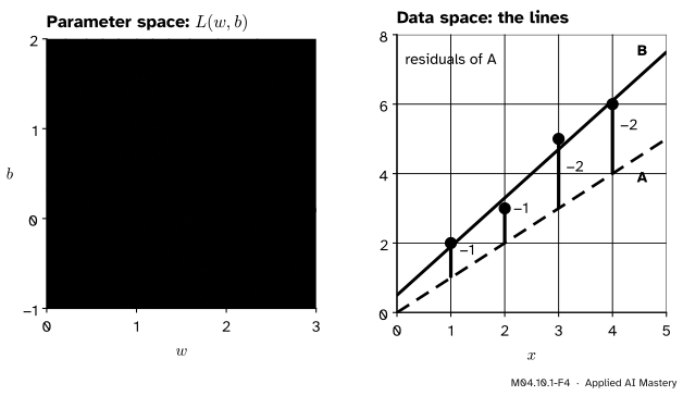
The four points stay fixed. The inputs of this function are \(w\) and \(b\). Line A, with \({w = 1}\) and \({b = 0}\), predicts 1, 2, 3, 4, so its residuals are \({-1, -1, -2, -2}\), their squares 1, 1, 4, 4, and
\[
L(1, 0) = \frac{1 + 1 + 4 + 4}{4} = 2.5 .
\]
Line B, with \({w = 1.4}\) and \({b = 0.5}\), predicts 1.9, 3.3, 4.7, 6.1. Its residuals are \({-0.1, 0.3, -0.3, 0.1}\), their squares 0.01, 0.09, 0.09, 0.01, and \({L(1.4, 0.5) = 0.2/4 = 0.05}\).
M04.10.1-F4
Each point of the map on the left is a line on the right, and its height on the map is that line’s loss. Line A misses every point from below; line B, at the star, nearly fits.
Multiplying out gives the loss as one formula. Each term of the sum expands like this:
\[
\begin{aligned}
&(w x_i + b - y_i)^2 \\
&\quad = x_i^2 w^2 + 2 x_i w b + b^2 \\
&\qquad - 2 x_i y_i w - 2 y_i b + y_i^2 .
\end{aligned}
\]
Adding the four terms needs five sums over the points: \({\sum x_i = 10}\), \({\sum x_i^2 = 30}\), \({\sum x_i y_i = 47}\), \({\sum y_i = 16}\) and \({\sum y_i^2 = 74}\). The term \(b^2\) appears once per point, four times in all:
Check: \({L(1, 0)} = {7.5 - 23.5 + 18.5} = {2.5}\). Freeze \({b = 0}\) and the slice is \({7.5w^2 - 23.5w + 18.5}\), the running loss of M04.4: the one-parameter loss of this course is a single slice of this surface.
Code
First the table, with two nested loops and nothing else.
def f(x, y):return x**2+2* y**2grid = [-2, -1, 0, 1, 2]for y inreversed(grid): # the top row is y = 2, as on a mapprint(f"y = {y:2d}:", [f(x, y) for x in grid])
y =  2: [12, 9, 8, 9, 12]
y =  1: [6, 3, 2, 3, 6]
y =  0: [4, 1, 0, 1, 4]
y = -1: [6, 3, 2, 3, 6]
y = -2: [12, 9, 8, 9, 12]
NumPy builds the whole grid at once. np.meshgrid takes the \(x\) values and the \(y\) values and returns two arrays of the grid’s shape: one holds the \(x\) of every grid point, the other its \(y\). Arithmetic on them then works point by point. By default row i belongs to ys[i] and column j to xs[j], so the rows run from \({y = -2}\) upwards.
import numpy as npxs = np.array(grid)ys = np.array(grid)X, Y = np.meshgrid(xs, ys)Z = f(X, Y)print(Z)
Now the loss, on a fine grid: 31 values of \(w\) from 0 to 3 and 31 values of \(b\) from \(-1\) to 2, in steps of 0.1, so 961 lines in all. np.argmin finds the position of the smallest value, counting through the array row by row, and np.unravel_index turns that count back into a row and a column.
x = np.array([1.0, 2.0, 3.0, 4.0])y = np.array([2.0, 3.0, 5.0, 6.0])def loss(w, b):"""The mean squared error of the line w x + b on the four points."""return np.mean((w * x + b - y) **2)ws = np.linspace(0, 3, 31)bs = np.linspace(-1, 2, 31)W, B = np.meshgrid(ws, bs) # rows follow b, columns follow wL =7.5* W**2+5* W * B + B**2-23.5* W -8* B +18.5k = np.argmin(L)row, col = np.unravel_index(k, L.shape)print(L.size, "grid values")print(f"lowest: w = {ws[col]:.1f}, b = {bs[row]:.1f}, L = {L[row, col]:.3f}")print(f"from the residuals: L = {loss(ws[col], bs[row]):.3f}")
961 grid values
lowest: w = 1.4, b = 0.5, L = 0.050
from the residuals: L = 0.050
The multiplied-out formula and the mean of squared residuals agree, and the lowest of the 961 grid values is line B. A grid is evidence, not proof: it looks at 961 lines only, and the true lowest point could lie between them. Lesson 4 finds the lowest point exactly.
Explore
This module’s interactive, the slope compass, lives in lesson M04.10.3. Choose the running bowl there and drag the point across the contour map: the side panels draw the two slices through the point, and the read-out gives its height.
Pitfalls
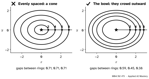
M04.10.1-F5
Wrong beside right. Rings at heights 2, 4, 6 and 8 drawn evenly spaced belong to a cone, whose height grows evenly with distance. The bowl’s rings crowd together as it gets steeper.
“Contour lines at equal steps of height are equally far apart.”
Only for a function that climbs at an even rate, like a cone. The bowl gets steeper as you go out, so each extra step of 2 in height comes sooner: along \(x\) its rings at heights 2, 4, 6 and 8 are 0.59, 0.45 and 0.38 apart. Read spacing as steepness, never as height. A loss map is read the same way: crowded lines mark the directions in which the loss is most sensitive to the parameters.
“Freezing an input gives a contour line.”
Freezing an input leaves a slice, a graph of height against the other input, such as \({x^2 + 2}\). Freezing the output gives a contour line, a curve in the plane of the inputs along which the height never changes. A slice has slopes; a contour line, by definition, is level.
“The lowest value on my grid is the lowest point of the function.”
A grid sees only its own points. With steps of 0.5 instead of 0.1, the best grid value of the loss is 0.125, shared by two lines, \({(w, b) = (1.5, 0)}\) and \({(1.5, 0.5)}\), and np.argmin returns the first one it meets. Neither is the bottom, whose loss is 0.05. A grid also grows fast: ten parameters with ten values each make ten billion points. Exact methods (lesson 4) and methods that follow slopes (ML01.5) take its place.
Check yourself
Recall
1. What does a function of two inputs give at each point of the plane, and what is its graph?
Show answer
One number, read as a height. Its graph is the surface of points \({(x, y, z)}\) with \({z = f(x, y)}\).
2. What is the contour line of \(f\) at height \(c\)?
Show answer
The set of points \((x, y)\) in the plane where \({f(x, y) = c}\): on a map, the line joining the points of that height.
3. Contour lines at equal steps of height lie close together in one part of a map. What does that tell you?
Show answer
The ground is steep there: the height changes a lot over a short distance.
4. What do you get when you freeze \({y = 1}\) in \({f(x, y) = x^2 + 2y^2}\)?
Show answer
The slice \({f(x, 1) = x^2 + 2}\): an ordinary function of \(x\), whose graph is a parabola.
5. For the loss \({L(w, b)}\) of a line through four points, which numbers are the inputs and which stay fixed?
Show answer
The inputs are the slope \(w\) and the intercept \(b\). The four points, inputs \(x_i\) and targets \(y_i\), stay fixed.
Exercises
1.★ For the running bowl, find \({f(2, -1)}\) and \({f(-1, 2)}\), and the points where its contour line at height 18 crosses the two axes.
Show solution
\({f(2, -1)} = {4 + 2} = {6}\) and \({f(-1, 2)} = {1 + 8} = {9}\). At height 18: on the \(x\) axis \({x^2 = 18}\), so \({x = \pm\sqrt{18} = \pm 3\sqrt{2} \approx \pm 4.24}\); on the \(y\) axis \({2y^2 = 18}\), so \({y = \pm 3}\).
2.★★ Describe the contour lines of \({h(x, y) = x^2 - y^2}\) at heights \(-1\), 0 and 1, and the slices through \({y = 0}\) and \({x = 0}\).
Show solution
Height 0: \({x^2 = y^2}\), so \({y = x}\) or \({y = -x}\), two straight lines crossing at the origin. Height 1: \({x^2 - y^2 = 1}\) crosses the \(x\) axis at \({\pm 1}\) and never meets the \(y\) axis, since \({-y^2 = 1}\) is impossible: a curve in two pieces opening left and right. Height \(-1\): the same curve turned a quarter turn, crossing the \(y\) axis at \({\pm 1}\) and opening up and down.
The slice through \({y = 0}\) is \({h(x, 0) = x^2}\), a parabola opening upwards: a valley. The slice through \({x = 0}\) is \({h(0, y) = -y^2}\), a parabola opening downwards: a ridge. A surface that is a valley one way and a ridge the other is a saddle; lesson 4 returns to it.
3.★★★ For the two-parameter loss: (a) compute \({L(1, 1)}\) and \({L(2, -1)}\) from the residuals, and say what the two answers mean together; (b) write the slice \({w = 1}\) as a function of \(b\), find its lowest point, and decide whether that is the lowest point of the whole surface.
Show solution
(a) The line \({w = 1}\), \({b = 1}\) predicts 2, 3, 4, 5; its residuals are 0, 0, \(-1\), \(-1\) and \({L(1, 1)} = {(0 + 0 + 1 + 1)/4} = {0.5}\). The line \({w = 2}\), \({b = -1}\) predicts 1, 3, 5, 7; its residuals are \(-1\), 0, 0, 1 and \({L(2, -1) = 0.5}\) too. The two points lie on the same contour line of the loss, at height 0.5: by this loss the two lines are equally good.
(b) Put \({w = 1}\) into the multiplied-out formula:
Its derivative \({2b - 3}\) is zero at \({b = 1.5}\), negative before and positive after, so by the first-derivative test (M04.4.1) this is the slice’s lowest point, of height \({2.25 - 4.5 + 2.5 = 0.25}\). It is not the lowest point of the surface: line B has loss 0.05. The best line among those of slope 1 is not the best line.
Summary card
A function of two inputs is a landscape: a surface from the side, contour lines from above, and slices when one input is frozen.
M04.10.1-F1
One bowl, seen two ways.
Function: one height \({f(x, y)}\) for each point \((x, y)\) of the plane.
Contour line at height \(c\): the points where \({f(x, y) = c}\). Crowded lines mean steep ground.
Slice: freeze one input, as in \({f(x, 1) = x^2 + 2}\), and an ordinary curve is left.
The bowl: its rings \({x^2 + 2y^2 = c}\) are ellipses with half-widths \(\sqrt{c}\) and \(\sqrt{c/2}\).
The loss:\({L(w, b)}\) is a function of the line’s two numbers; on a grid it is lowest, 0.05, at \({(1.4, 0.5)}\).
Sources and next steps
Sources. Each was opened and checked against this lesson on 12 November 2026.
Gilbert Strang and Edwin Herman, Calculus Volume 3 (OpenStax), Section 4.1: the definitions of a function of two variables, of a level curve and a contour map, and of a vertical trace, the name used there for a slice. Its Example 4.2 finds that the level curves of \({x^2 + y^2}\) are circles of increasing radius.
NumPy 2.5 reference, numpy.meshgrid: Cartesian ('xy') indexing is the default, so for inputs of lengths \(M\) and \(N\) the outputs have shape \({(N, M)}\), one row for each value of the second input.
NumPy 2.5 reference, numpy.argmin: with no axis given it indexes the flattened array and returns the first occurrence of the minimum, and its examples pair it with numpy.unravel_index.
Next.M04.10.2 Partial derivatives measures the slope of each slice: how fast the height changes when only one input moves.