Fix the left end of an integral and let the right end move, and the area becomes a function of x. Find it from rectangles and triangles, build it as a running total with numpy.cumsum, and notice that its slope is always the height of the curve.
Define the area function A(x), the integral of f(t) dt from a fixed start a to a moving end x, and explain why the variable inside is written t.
Find the area function of a constant and of f(t) = t from rectangles and triangles.
Build an area function from data as a running total of thin strips with numpy.cumsum, and read the running trip’s distance so far from it.
Explain why A(a) = 0 and why the area function falls where f is negative.
Measure the slope of an area function and compare it with the height of the curve.
In review. The maths and code on this page are checked by automated tests on every change, but an independent reader has not signed it off yet. Spot a mistake or a confusing step? Tell us.
The question
A cart’s speedometer is read every second, but nothing records how far the cart has gone. The distance covered by time \(x\) is the area under the speed curve from 0 to \(x\). Let \(x\) slide on and the area changes with it, so the area is a function of \(x\). What does its graph look like, and how fast does it climb?
Intuition
Until now an integral has been one number: the area under a curve between two fixed ends (M04.5.2). Now keep the left end fixed and let the right end move. Each position \(x\) of the right end gives one area. A rule that turns each number into one number is a function, so the area is a function of \(x\): the area function of the curve.
M04.6.1-F1
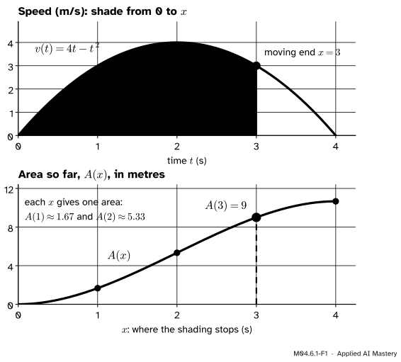
The running trip, a cart whose speed is \({v(t) = 4t - t^2}\) metres per second (an invented example). Top: the area under the speed curve from 0 to the moving end \(x\) is the distance covered by time \(x\); at \({x = 3}\) it is 9 metres. Bottom: that area for every \(x\), drawn as a curve. Its height at 3 is the shaded area, 9.
Three things show in the picture.
At the start nothing is shaded, so the area function begins at 0.
It climbs fastest where the curve is highest. Near \({t = 2}\), where the cart is fastest, each extra moment adds the most area.
It is nearly flat where the curve is low. Near the start and the end the cart is slow, and the area hardly grows.
So the steepness of the lower curve seems to follow the height of the upper one. That observation is where this lesson ends, and the next lesson proves it.
Area functions are common in machine learning too. The area under a probability density to the left of \(x\) is the cumulative distribution function (M06.6), and the next lesson finds one inside GELU, an activation function of transformer networks.
Build it up
Step 1. Fix the start and let the end move. Write the area from a fixed start \(a\) to a moving end \(x\) as
\[
A(x) = \int_a^x f(t)\,dt .
\]
The letter inside, \(t\), is the point that runs along the axis from \(a\) to \(x\) while the strips are added up, like the loop variable in for t in .... Its name does not matter: \({\int_a^x f(u)\,du}\) is the same number. It only must not be \(x\), which already names the right end.
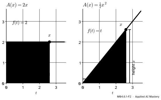
Step 2. A constant height gives a rectangle. Take \({f(t) = 2}\) and start at \({a = 0}\). The region from 0 to \(x\) is a rectangle of width \(x\) and height 2, so \({A(x) = 2x}\). Its graph is a straight line whose slope, 2, is the height of \(f\).
Step 3. A sloping line gives a triangle. Take \({f(t) = t}\), again from 0. For \({x > 0}\) the region is a right triangle with base \(x\) and height \(x\), so \({A(x) = \tfrac12 x^2}\). At \({x = 1, 2, 3, 4}\) this gives 0.5, 2, 4.5 and 8: doubling \(x\) multiplies the area by four. By the power rule (M04.3.1) the slope of \({\tfrac12 x^2}\) is \(x\), which is again the height of \(f\) at \(x\).
M04.6.1-F2
Two area functions found by geometry. Under a constant height the region is a rectangle; under the line \({f(t) = t}\) it is a triangle. The titles, in the colour of the area function, give the area for every \(x\).
Step 4. No shape formula: add thin strips. The trip’s speed curve is neither a rectangle nor a triangle. Cut the time from 0 to \(x\) into strips of width \({\Delta t}\), give each strip the height of the curve at its left edge, and keep a running total, as in M04.5.1. With strips one second wide the heights are the speeds 0, 3, 4 and 3, and the running totals at \({x = 1, 2, 3, 4}\) are 0, 3, 7 and 10 metres. The cart’s position, \({s(t) = 2t^2 - \tfrac13 t^3}\) metres, whose slope is the speed (M04.3.1), says how far it has really gone: about 1.67, 5.33, 9 and 10.67 metres. While the speed rises, each left edge is the lowest point of its strip, so the totals fall behind; once the speed falls, they catch up a little. Thinner strips close the gap, and a running total is exactly what numpy.cumsum computes.
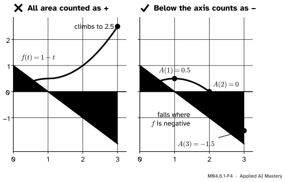
Step 5. Below the axis the area function falls. Area below the axis counts as negative (M04.5.3), so where \(f\) is negative each new strip takes something away. Take \({f(t) = 1 - t}\) from 0. Up to \({x = 1}\) the region is a trapezoid with parallel sides 1 and \({1 - x}\), so \({A(x) = x - \tfrac12 x^2}\). Past 1 a triangle below the axis, of area \({\tfrac12 (x - 1)^2}\), is taken from the 0.5 above it, which gives the same formula. So \(A\) climbs to 0.5 at \({x = 1}\), is back to 0 at \({x = 2}\), and reaches \({-1.5}\) at \({x = 3}\).
Step 6. Compare slopes with heights. In every case the slope of \(A\) at \(x\) has been the height of \(f\) at \(x\): 2 for the rectangle, \(x\) for the triangle, \({1 - x}\) for the trapezoid. For the trip, the code below measures the slope of the running total at 1, 2 and 3 seconds and finds 3, 4 and 3 metres per second, the speeds there.
The formal statement
NoteDefinition: area function
Let \(f\) be continuous on an interval that contains the point \(a\). The area function of \(f\) from \(a\) is
\[
A(x) = \int_a^x f(t)\,dt
\]
for every \(x\) in the interval. When \({x < a}\) the integral runs backwards, and by the rule for reversed limits (M04.5.3) it equals \({-\int_x^a f(t)\,dt}\).
Three facts follow from the rules of M04.5.3.
Fact 1: it starts at zero.\({A(a) = \int_a^a f(t)\,dt = 0}\), because an interval of width 0 holds no area.
Fact 2: a change in \(A\) is the area in between. For any two points \(c\) and \(x\) of the interval, splitting the integral at \(c\) gives
In words: the change in the area function between two points is the area between them. Because of the rule for reversed limits, the split holds whatever the order of \(a\), \(c\) and \(x\). The next lesson’s proof starts from this line.
Fact 3: \(A\) rises where \(f\) is positive and falls where \(f\) is negative. Take \({c < x}\) and suppose \({f(t) > 0}\) for every \(t\) from \(c\) to \(x\). A continuous function on a closed interval has a least value there (the extreme value theorem, M04.4.3); call it \(m\), so \({m > 0}\). Every height on the stretch is at least \(m\), so the comparison rule gives
By Fact 2 this is \({A(x) - A(c)}\), so \({A(x) > A(c)}\): the area function has risen. If instead \(f\) is negative on the whole stretch, the same steps with its greatest value \({M < 0}\) give \({A(x) < A(c)}\).
Units. If \(t\) is in seconds and \(f\) in metres per second, a strip of width \({\Delta t}\) and height \(f\) has an area in metres. So the area function of a rate is an amount: the trip’s area function is a distance.
Go deeper: what changes if the start moves
Let \(A\) start at \(a\) and \(B\) start at \(b\), for the same \(f\). Splitting the integral that defines \(A\) at \(b\) gives
The first term is one fixed number; it does not depend on \(x\). So two area functions of the same \(f\) differ by a constant, and their graphs are the same curve slid up or down. For \({f(t) = t}\), starting at 0 gives \({\tfrac12 x^2}\) and starting at 1 gives \({\tfrac12 x^2 - \tfrac12}\). This constant comes back as \(C\) in lesson M04.6.3.
Worked example
The area function of \({f(t) = t}\) from 0, and its slope at 2.
The areas. For \({x > 0}\) the region under the line from 0 to \(x\) is a right triangle with base \(x\) and height \({f(x) = x}\). Half the base times the height gives \({A(x) = \tfrac12 x^2}\), so \({A(1) = 0.5}\), \({A(2) = 2}\) and \({A(3) = 4.5}\).
For a negative end, say \({x = -2}\), the limits run backwards: \({A(-2) = -\int_{-2}^{0} t\,dt}\). Between \({-2}\) and 0 the line lies below the axis and encloses a triangle of area 2, so \({\int_{-2}^{0} t\,dt = -2}\) and \({A(-2) = 2}\). The formula agrees, since \({\tfrac12 (-2)^2 = 2}\), so \({A(x) = \tfrac12 x^2}\) holds for every \(x\).
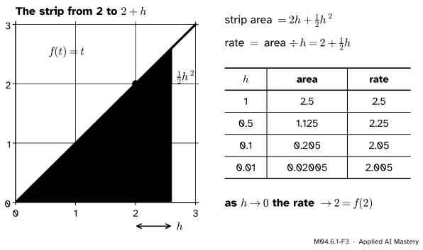
The slope at 2. The slope of \(A\) at 2 is the limit of a difference quotient (M04.2.1). Moving the end from 2 to \({2 + h}\), with \({h > 0}\), adds the strip shown below: a rectangle of height 2 and width \(h\), with a small triangle whose two short sides are both \(h\) on top.
M04.6.1-F3
The strip added when the end moves from 2 to \({2 + h}\): a rectangle of area \({2h}\) and a small triangle of area \({\tfrac12 h^2}\). Divided by \(h\), the area gives the rate at which \(A\) grows, \({2 + \tfrac12 h}\), which tends to 2.
The formula gives the same strip: \({\tfrac12 (2 + h)^2 - 2 = \tfrac12 (4 + 4h + h^2) - 2}\), which is \({2h + \tfrac12 h^2}\). Because the formula holds for every \(x\), this algebra also works for \({h < 0}\). As \(h\) shrinks to 0 the quotient tends to 2, which is \({f(2)}\).
Look at where each part came from. The rectangle supplies the 2, the height of \(f\). The little triangle supplies the \({\tfrac12 h}\), and it vanishes as the strip gets thinner. That is the whole idea of the next lesson, in one example.
Code
First from scratch, with a plain loop: the running total of the trip’s one-second strips, each taking the speed at its left edge.
def v(t):"""The running trip's speed, in metres per second."""return4* t - t **2def s(t):"""The cart's position: how far it has really gone, in metres."""return2* t **2- t **3/3dt =1.0totals = [0.0] # the area function at t = 0, 1, 2, 3, 4for k inrange(4): left_height = v(k * dt) # the strip from k to k + 1 takes its left-edge height totals.append(totals[-1] + left_height * dt)print("running totals:", totals)print("true distance: ", [round(s(k), 4) for k inrange(5)])
Now thin strips with NumPy. np.cumsum turns a list of strip areas into the list of running totals, and putting 0 in front makes the first entry the area up to the start. Each strip takes the speed at its middle, the midpoint rule of M04.5.2, which is far more accurate than the left edge.
import numpy as npdt =0.001t = np.linspace(0, 4, 4001) # the strip edges: 0, 0.001, ..., 4 secondsmid = t[:-1] + dt /2# the middle of each stripA = np.concatenate([[0.0], np.cumsum(v(mid) * dt)]) # A[k] is the area from 0 to t[k]for x in (1, 2, 3, 4): k =round(x / dt)print(f"A({x}) = {A[k]:.5f} s({x}) = {s(x):.5f}")
The running totals agree with the true distance to within a millionth of a metre: the trip’s area function is its position. Finally, measure the slope of the area function with a central difference (M04.2.4), stepping ten strips each way, and set it beside the height of the speed curve.
for x in (1, 2, 3): k, m =round(x / dt), 10# m strips each way: h = 0.01 seconds slope = (A[k + m] - A[k - m]) / (2* m * dt)print(f"slope of A at {x}: {slope:.4f} speed v({x}) = {v(x):.4f}")
slope of A at 1: 3.0000   speed v(1) = 3.0000
slope of A at 2: 4.0000   speed v(2) = 4.0000
slope of A at 3: 3.0000   speed v(3) = 3.0000
At every point tried, the slope of the area function is the height of the curve. A table is evidence, not proof; the proof is the next lesson.
Explore
This module’s interactive, the area accumulator, lives in the next lesson. Drag the moving end along the graph of a function and watch the area function being traced below it, rising where the curve is above the axis and falling where it is below.
Pitfalls
M04.6.1-F4
Wrong beside right, for \({f(t) = 1 - t}\). Counting every piece of area as positive gives a curve that only climbs. The area function counts the area below the axis as negative, so it falls once \(f\) is negative.
“Area can’t be negative, so the area function only goes up.”
The integral counts area below the axis as negative (M04.5.3), so \(A\) falls wherever \(f\) is negative. For \({f(t) = 1 - t}\), \({A(3) = -1.5}\), while the two shaded triangles have areas 0.5 and 2, which add up to 2.5. Both numbers have uses; lesson M04.6.4 needs the second kind for the total distance of a trip. But only the signed one is the area function.
“\({A(x)}\) is the height of the curve at \(x\).”
\({A(x)}\) is an area, and it depends on \(f\) all the way from \(a\) to \(x\). At the start it is 0 whatever \({f(a)}\) is. For the trip, \({A(1) \approx 1.67}\) metres while the height there is \({v(1) = 3}\) metres per second: not even the same units. What the height of \(f\) controls is the slope of \(A\).
“I’ll write the area function as \({\int_a^x f(x)\,dx}\).”
Then \(x\) means two things at once: the right end of the interval and the point running across it. It is the same mistake as writing for x in range(x) in Python. Use another letter, such as \(t\), for the running point.
“np.cumsum(v) gives the distance.”
It adds speeds, not areas. Each height must be multiplied by the strip width first: np.cumsum(v * dt). With strips a thousandth of a second wide, forgetting dt makes every total a thousand times too large.
Check yourself
Recall
1. In \({A(x) = \int_a^x f(t)\,dt}\), which end is fixed and which moves?
Show answer
The left end \(a\) is fixed and the right end \(x\) moves. The area function gives the area for each position of the right end.
2. What is \({A(a)}\), and why?
Show answer
0, because the interval from \(a\) to \(a\) has width 0 and holds no area.
3. What is the area function of \({f(t) = 5}\) from 0?
Show answer
\({A(x) = 5x}\): the region is a rectangle of height 5 and width \(x\).
4. For \({f(t) = t}\) from 0, what is \({A(4)}\)?
Show answer
8: the region is a triangle with base 4 and height 4, so its area is \({\tfrac12 \times 4 \times 4}\).
5. Where does an area function fall?
Show answer
Where \(f\) is negative, because area below the axis counts as negative and each new strip takes something away.
Exercises
1.★ Let \({f(t) = 3}\) and start at \({a = 2}\). Find \({A(x)}\), then \({A(5)}\) and \({A(1)}\).
Show solution
For \({x > 2}\) the region is a rectangle of height 3 and width \({x - 2}\), so \({A(x) = 3(x - 2)}\) and \({A(5) = 9}\). For \({x = 1}\) the limits run backwards: \({A(1) = -\int_1^2 3\,dt = -3 \times 1 = -3}\). The formula gives the same, \({3\,(1 - 2) = -3}\), so \({A(x) = 3(x - 2)}\) for every \(x\).
2.★★ Let \({f(t) = 2t}\) and start at \({a = 1}\). Find \({A(x)}\) for \({x > 1}\) by geometry, check that its slope is \({f(x)}\), and find \({A(3)}\).
Show solution
Between \({t = 1}\) and \({t = x}\) the region is a trapezoid. Its parallel sides are the heights \({f(1) = 2}\) and \({f(x) = 2x}\), and its width is \({x - 1}\). The area of a trapezoid is the average of the parallel sides times the width:
By the power rule its slope is \({2x}\), which is \({f(x)}\). And \({A(3) = 9 - 1 = 8}\). The check \({A(1) = 1 - 1 = 0}\) agrees with Fact 1.
3.★★★ Let \(A\) be the area function of the running curve \({f(t) = t^2}\) from 0, so that \({A(1) = \tfrac13}\) (M04.5.2). For \({h > 0}\), show without finding a formula for \(A\) that
By Fact 2, \({A(1 + h) - A(1) = \int_1^{1+h} t^2\,dt}\), the area of the strip from 1 to \({1 + h}\). On that strip \({t^2}\) rises, so every height lies between \({1^2 = 1}\) and \({(1 + h)^2}\). By the comparison rule the strip’s area lies between the areas of the two rectangles with those heights:
\[
\begin{aligned}
1 \cdot h \;&\le\; \int_1^{1+h} t^2\,dt \\
&\le\; (1 + h)^2\, h .
\end{aligned}
\]
Dividing by \({h > 0}\) gives the inequality. As \(h\) shrinks to 0 the right-hand side tends to 1, so the quotient is squeezed between 1 and a number that tends to 1 (the squeeze theorem, M04.1.2). Its limit from the right is 1, which is \({f(1)}\). The next lesson makes this argument work for every continuous \(f\) and from both sides.
Summary card
The area up to a moving end is a function of that end, and its slope is the height.
M04.6.1-F1
Area so far, as a function of where it stops.
Definition.\({A(x) = \int_a^x f(t)\,dt}\), and \({A(a) = 0}\).
By geometry.\({f = c}\) gives \({A(x) = c\,(x - a)}\); \({f(t) = t}\) from 0 gives \({\tfrac12 x^2}\).
Change.\({A(x) - A(c) = \int_c^x f(t)\,dt}\): rising where \({f > 0}\), falling where \({f < 0}\).
From data.np.concatenate([[0], np.cumsum(f(mid) * dt)]).
Observed. The slope of \(A\) at \(x\) is \({f(x)}\), proved in the next lesson.
Sources and next steps
Sources. Each was opened and checked against this lesson on 12 November 2026.
Gilbert Strang and Edwin Herman, Calculus Volume 1 (OpenStax), Section 5.3: Theorem 5.4 is stated for \({F(x) = \int_a^x f(t)\,dt}\), a function of the upper limit, with \(f\) continuous on \({[a, b]}\).
Matt Boelkins, Active Calculus, Section 5.2: the integral function \({A(x) = \int_c^x f(t)\,dt}\) with a fixed start \(c\), and \({A(c) = 0}\).
David Jerison, MIT 18.01 Single Variable Calculus (Fall 2006), Lecture 19 notes: the additive property \({\int_a^b + \int_b^c = \int_a^c}\), and the definition of reversed limits that makes it hold for \(a\), \(b\), \(c\) in any order.
NumPy documentation, numpy.cumsum (version 2.5): the cumulative sum of the elements along an axis, with the note that the last running total, cumsum(a)[-1], may differ from sum(a) for floating-point values.