A recipe for exact optimisation: write the quantity as a function of one variable, find its critical points, and compare them with the ends of the interval. Then derive two results data science uses daily: the mean minimises squared deviations, and 7 heads in 10 tosses make 0.7 the most likely chance of heads.
Find the largest and smallest values of a continuous function on a closed interval by comparing its critical points with the endpoints.
State the extreme value theorem and explain why both a closed interval and continuity are needed.
Derive that the mean minimises the sum of squared deviations, and find the best slope of the running loss by the same steps.
Derive the maximum likelihood estimate for a coin from its log-likelihood, and explain why taking logarithms keeps the answer.
In review. The maths and code on this page are checked by automated tests on every change, but an independent reader has not signed it off yet. Spot a mistake or a confusing step? Tell us.
The question
Two of the most used numbers in data science are answers to optimisation problems. The mean of some measurements is the centre that makes the squared errors smallest. And a coin that showed 7 heads in 10 tosses gets the estimate 0.7 because no other chance of heads makes those tosses more likely. Why exactly those numbers? And when a quantity can only vary over an interval, where can its best value hide?
From the last lesson
1. State the second-derivative test.
Show answer
If \({f'(c) = 0}\) and \({f''(c) > 0}\), \(c\) is a local minimum; if \({f''(c) < 0}\), a local maximum; if \({f''(c) = 0}\), the test says nothing.
2. Why is \({w = 47/30}\) the lowest point of the running loss, not just a local minimum?
Show answer
\({L''(w) = 15 > 0}\) for every \(w\), so \(L\) is convex, and a flat point of a convex function is its lowest point.
Intuition
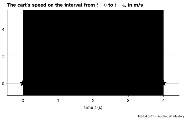
When is the cart of the running trip fastest, and when is it slowest? Its speed is \({v(t) = 4t - t^2}\) metres per second, and the trip lasts from \({t = 0}\) to \({t = 4}\).
M04.4.3-F1
On an interval the extremes sit in two kinds of places: at a flat point inside, like the top speed, or at an end, like the standing starts, where the slope is far from zero.
The fastest moment is a flat top inside the interval, where \({v'(2) = 0}\): the territory of the last two lessons. The slowest moments are the two ends, where the cart stands still. There the slope is 4 or \({-4}\), not 0. Fermat’s theorem only speaks about points with neighbours on both sides, so it says nothing about the ends. A search for the best value must therefore look in both places: at the flat points inside, and at the ends.
Build it up
Step 1. One quantity, one variable. Write what you want to make large or small as a function of a single variable: the speed as a function of time, a loss as a function of a weight, a probability as a function of an unknown chance.
Step 2. The allowed values. Decide which values the variable may take. Usually that is an interval: time from 0 to 4, a chance between 0 and 1.
Step 3. The candidates. By Fermat’s theorem, a largest or smallest value at an inside point sits at a critical point. Any other extreme must be at an end. So the candidates are the critical points inside the interval and the two ends.
Step 4. Compare. Work out the function at every candidate. The largest value is the maximum and the smallest is the minimum.
One question is left: does a largest value exist at all? The next section answers it.
The formal statement
NoteTheorem: the extreme value theorem
A function that is continuous on a closed interval \({[a, b]}\) takes a largest value and a smallest value somewhere on that interval.
The theorem is stated here without proof, which needs a careful study of the real numbers. Both conditions matter. On the open interval \({(0, 1)}\) the function \({f(x) = x}\) climbs towards 1 but never gets there, so it has no largest value. And a function with a jump can skip over its would-be top.
NoteThe closed-interval method
To find the largest and smallest values of a function \(f\) that is continuous on \({[a, b]}\):
find the critical points of \(f\) inside \({(a, b)}\);
evaluate \(f\) there and at both ends, \(a\) and \(b\);
the largest of these values is the maximum, the smallest is the minimum.
Why it works. By the extreme value theorem the maximum is taken at some point \(c\). If \(c\) is inside the interval, \(f\) has a local maximum there, so \(c\) is a critical point (Fermat). Otherwise \(c\) is an end. Either way \(c\) is on the list. The same argument holds for the minimum.
Result 1: the mean minimises the squared deviations. Given numbers \({y_1, \dots, y_n}\), which single number \(c\) is closest to all of them, in the sense of the smallest sum of squared deviations?
\[
S(c) = \sum_{i=1}^{n} (y_i - c)^2 .
\]
Differentiate one term with the chain rule (M04.3.4): the outside square gives \({2(y_i - c)}\) and the inside \({y_i - c}\) has slope \({-1}\). Summing the terms,
This is zero exactly when \({nc}\) equals the sum of the \({y_i}\), that is at
\[
c = \frac{1}{n} \sum_{i=1}^{n} y_i ,
\]
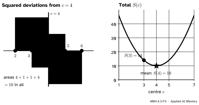
the mean, written \({\bar{y}}\). Differentiating again, \({S''(c) = 2n > 0}\), so \(S\) is convex and the mean is its lowest point over all numbers \(c\) (M04.4.2). For the running targets 2, 3, 5 and 6 the mean is \({16/4 = 4}\), and \({S(4) = 4 + 1 + 1 + 4 = 10}\).
M04.4.3-F3
The sum of squared deviations, drawn as squares. Any centre other than the mean makes the total area larger: at \({c = 3}\) the squares add up to 14.
The running loss, by the same steps. The mean squared error of the line \({\hat{y} = wx}\) on the four points (ML01.5.1) is \({L(w)} = {\frac{1}{4}\sum (wx_i - y_i)^2}\). One term differentiates to \({2(wx_i - y_i)x_i}\), so
using \({\sum x_i^2 = 1 + 4 + 9 + 16 = 30}\) and \({\sum x_i y_i} = {2 + 6 + 15 + 24} = {47}\). It is zero at \({w = 47/30 \approx 1.567}\), and \({L'' = 15 > 0}\) makes that the lowest point. The mean is the special case where every \({x_i}\) is 1: the best constant prediction.
Result 2: the most likely chance of heads. A coin with an unknown chance \(p\) of heads is tossed 10 times and shows 7 heads and 3 tails. The tosses are independent, so the probability of that exact sequence is
\[
p^7 (1 - p)^3 .
\]
Read as a function of \(p\), this is the likelihood. The maximum likelihood estimate is the \(p\) that makes it largest. Logarithms turn the product into a sum (M01.4), and since \({\ln}\) is increasing, the largest likelihood and the largest logarithm happen at the same \(p\). So maximise the log-likelihood, for \(p\) between 0 and 1,
\[
f(p) = 7\ln p + 3\ln(1 - p) .
\]
By the chain rule, \({\ln(1 - p)}\) has slope \({-1/(1 - p)}\). So
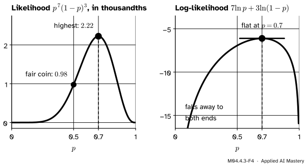
Both terms are negative, so \({f''(p) < 0}\): \(f\) is concave down on the whole interval, \({-f}\) is convex, and the flat point \({p = 0.7}\) is the highest point of \(f\). The answer is the share of heads seen. The likelihood there is \({0.7^7 \times 0.3^3} \approx {0.00222}\), more than twice the \({0.5^{10} \approx 0.00098}\) of a fair coin. If only the count of heads is recorded, every probability gains the factor \({\binom{10}{7} = 120}\) (M01.8), which does not move the peak.
M04.4.3-F4
The likelihood and its logarithm have different heights but the same peak, at \({p = 0.7}\), because the logarithm never changes the order of two numbers.
Maximum likelihood in general, for any model and data, is S02.3.
Worked example
Find the largest and smallest values of the running cubic \({g(x) = x^3 - 3x}\) on the interval \({[0, 3]}\).
Step 1: does an answer exist?\(g\) is a polynomial, so it is continuous, and \({[0, 3]}\) is closed. The extreme value theorem promises a largest and a smallest value.
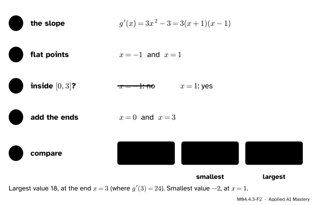
Step 2: critical points.\({g'(x)} = {3x^2 - 3} = {3(x + 1)(x - 1)}\) is zero at \({x = -1}\) and \({x = 1}\), and exists everywhere. Only \({x = 1}\) lies inside \({(0, 3)}\); \({x = -1}\) is not in the interval at all.
Step 3: the candidates. The critical point 1 and the two ends, 0 and 3.
Step 4: compare.\({g(0) = 0}\), \({g(1) = 1 - 3 = -2}\) and \({g(3) = 27 - 9 = 18}\). The largest is 18, at the end \({x = 3}\), where the slope \({g'(3) = 24}\) is far from zero. The smallest is \({-2}\), at \({x = 1}\).
M04.4.3-F2
The closed-interval method, step by step. The winner for the largest value is an end, which no search for flat points would ever find.
Code
From scratch, the closed-interval method is a few lines: a list of candidates and a comparison.
def g(x):return x**3-3* xdef closed_interval_method(f, critical_points, a, b):"""The largest and smallest values of f on [a, b], with the inputs where they happen.""" candidates = [a, b] + [c for c in critical_points if a < c < b] values = {x: f(x) for x in candidates} best_x =max(values, key=values.get) worst_x =min(values, key=values.get)return (best_x, values[best_x]), (worst_x, values[worst_x])print("g on [0, 3]: (largest at, value), (smallest at, value) =", closed_interval_method(g, [-1, 1], 0, 3))print("speed on [0, 4]:", closed_interval_method(lambda t: 4* t - t**2, [2], 0, 4))
g on [0, 3]: (largest at, value), (smallest at, value) = ((3, 18), (1, -2))
speed on [0, 4]: ((2, 4), (0, 0))
The two results, checked against a fine grid of candidates and against NumPy:
import numpy as npy = np.array([2.0, 3.0, 5.0, 6.0])x = np.array([1.0, 2.0, 3.0, 4.0])centres = np.linspace(0, 8, 8001)S = ((y[:, None] - centres) **2).sum(axis=0)print("best centre on the grid:", centres[S.argmin()], " np.mean:", y.mean(), " S there:", S.min())print("best slope, sum(x*y)/sum(x**2):", (x * y).sum() / (x**2).sum(), "= 47/30")p = np.linspace(0.001, 0.999, 999)log_likelihood =7* np.log(p) +3* np.log(1- p)print("most likely p on the grid:", p[log_likelihood.argmax()].round(3))print("likelihood at 0.7 and at 0.5:", round(0.7**7*0.3**3, 5), round(0.5**10, 5))
best centre on the grid: 4.0   np.mean: 4.0   S there: 10.0
best slope, sum(x*y)/sum(x**2): 1.5666666666666667 = 47/30
most likely p on the grid: 0.7
likelihood at 0.7 and at 0.5: 0.00222 0.00098
A grid is evidence, not proof: it only looks at the points it was given, and it can miss a narrow dip between them. The derivations above are the proof.
Explore
The descent explorer in lesson M04.4.4 searches for the bottom of the running loss step by step, the way a computer does when no formula like \({47/30}\) is available.
Pitfalls
M04.4.3-F5
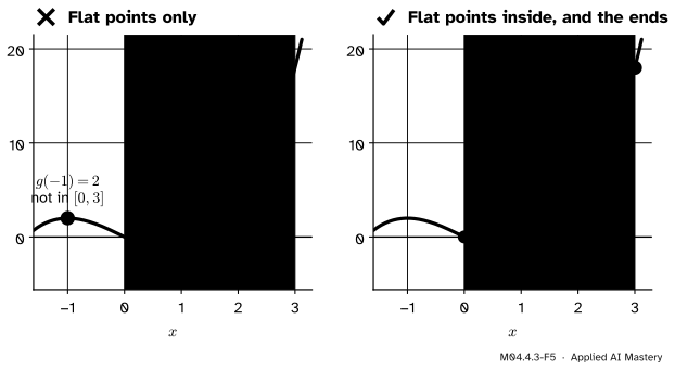
Wrong beside right. The flat points alone report a value from outside the interval and miss the true largest value, which sits at an end.
“The best value is where the derivative is zero.”
On an interval the best value can sit at an end, where the slope is anything. The running cubic on \({[0, 3]}\) is largest at \({x = 3}\), where \({g'(3) = 24}\), and the cart is slowest at the start and the finish. Always add the ends to the list.
“Every critical point of the function is a candidate.”
Only those inside the interval. \({x = -1}\) is a critical point of \(g\), but it is not in \({[0, 3]}\), so \({g(-1) = 2}\) says nothing about \(g\) on that interval.
“Any function on an interval has a largest value.”
Only a continuous function on a closed interval is promised one. \({f(x) = x}\) on the open interval \({(0, 1)}\) has none. The coin’s log-likelihood lives on an open interval too, which is why its peak was confirmed with the second derivative rather than by comparing ends.
Check yourself
Recall
1. State the extreme value theorem.
Show answer
A function that is continuous on a closed interval \({[a, b]}\) takes a largest and a smallest value on it.
2. Which points are the candidates in the closed-interval method?
Show answer
The critical points inside the interval, and the two ends.
3. Which number \(c\) minimises \({\sum (y_i - c)^2}\), and what is the smallest sum for 2, 3, 5, 6?
Show answer
The mean, \({\bar{y}}\). For 2, 3, 5 and 6 it is 4, and the sum is \({4 + 1 + 1 + 4 = 10}\).
4. Why may we maximise the log-likelihood instead of the likelihood?
Show answer
Because \({\ln}\) is increasing: a larger likelihood always has a larger logarithm, so both are largest at the same \(p\).
5. What is the maximum likelihood estimate of \(p\) after 7 heads in 10 tosses?
Show answer
\({p = 0.7}\), the share of heads seen.
Exercises
1.★ Find the largest and smallest speeds of the running trip, \({v(t) = 4t - t^2}\), on the interval \({[1, 4]}\).
Show solution
\({v'(t) = 4 - 2t}\) is zero only at \({t = 2}\), which is inside \({(1, 4)}\). The candidates are 1, 2 and 4: \({v(1) = 3}\), \({v(2) = 4}\) and \({v(4) = 0}\). The largest speed is 4 m/s at \({t = 2}\) and the smallest is 0 at the end \({t = 4}\).
2.★★ Cut a square of side \(x\) centimetres from each corner of a 12 cm by 12 cm sheet and fold up the sides to make an open box. Which \(x\) gives the largest volume?
Show solution
The base is a square of side \({u = 12 - 2x}\) and the height is \(x\), so \({V(x) = xu^2}\) for \({0 \leq x \leq 6}\). Since \({u' = -2}\), the product and chain rules give
which is zero at \({x = 6}\), an end, and at \({x = 2}\). The candidates give \({V(0) = 0}\), \({V(2) = 2 \times 8^2 = 128}\) and \({V(6) = 0}\). The largest volume is 128 cm³, with \({x = 2}\).
3.★★★ A coin shows \(k\) heads in \(n\) tosses. Show that the maximum likelihood estimate is \({p = k/n}\), including the cases \({k = 0}\) and \({k = n}\).
Show solution
The likelihood is \({p^k (1 - p)^{n - k}}\) on \({[0, 1]}\). If \({0 < k < n}\), it is 0 at both ends and positive inside, so the maximum is inside, where the log-likelihood \({k \ln p + (n - k)\ln(1 - p)}\) has slope \({k/p - (n - k)/(1 - p)}\). Setting this to zero gives \({k(1 - p) = (n - k)p}\), so \({k = np}\) and \({p = k/n}\); its second derivative is negative, so this is the highest point. If \({k = 0}\) the likelihood is \({(1 - p)^n}\), whose slope \({-n(1 - p)^{n - 1}}\) is negative inside the interval, so it is largest at the end \({p = 0 = k/n}\). If \({k = n}\) it is \({p^n}\), increasing, largest at the end \({p = 1 = k/n}\). In the last two cases the answer is an end, exactly as the closed-interval method warns.
Summary card
On an interval, the extremes are at flat points inside or at the ends.
M04.4.3-F1
Flat inside, or at an end.
Extreme value theorem: continuous on \({[a, b]}\) means a largest and a smallest value exist.
Closed-interval method: compare \(f\) at the critical points inside and at both ends.
The mean minimises \({\sum (y_i - c)^2}\); the running loss is lowest at \({w = 47/30}\).
Maximum likelihood for \(k\) heads in \(n\) tosses: \({p = k/n}\); for 7 in 10, 0.7.
Sources and next steps
Sources. Each was opened and checked against this lesson on 12 November 2026.
Gilbert Strang and Edwin Herman, Calculus Volume 1 (OpenStax), Section 4.3: the extreme value theorem (Theorem 4.1), absolute extrema lie at endpoints or critical points (Theorem 4.3), and the problem-solving strategy of evaluating the function at the endpoints and the critical points and comparing.
Matthew Boelkins, Active Calculus, Section 3.5, “Global optimization”: the extreme value theorem (Subsection 3.5.2) and the method of Note 3.5.2.
David Jerison, MIT OpenCourseWare 18.01SC, Session 29, “Optimization Problems”: extreme values are found at the boundaries of the range of options or where the graph levels out.
Jeremy Orloff and Jonathan Bloom, Maximum Likelihood Estimates, MIT OpenCourseWare 18.05, Class 10. Section 3 defines the maximum likelihood estimate and works a coin (55 heads in 100 tosses gives 0.55, the share of heads); Section 3.1 notes that, since ln is increasing, the likelihood and the log-likelihood have the same maximum.