When no antiderivative exists: Simpson’s rule and quad
The bell curve has no antiderivative built from elementary functions, so its areas must be computed numerically. Derive Simpson’s rule from a parabola through three samples, see why it is exact for cubics and why its error falls sixteenfold when the strips double, then use simpson and quad.
Explain why some areas, such as those under the bell curve, must be computed numerically even though the area function exists.
Derive the weights 1, 4, 1 of Simpson’s rule from the parabola through three equally spaced samples, and assemble the composite rule.
Show that Simpson’s rule is exact for cubics, and predict that doubling the strips divides its error by about 16, against 4 for the trapezoid rule.
Compute the normal probabilities 0.683, 0.954 and 0.997 with scipy.integrate.simpson and quad, and read quad’s error estimate critically.
In review. The maths and code on this page are checked by automated tests on every change, but an independent reader has not signed it off yet. Spot a mistake or a confusing step? Tell us.
The question
About 68% of a normal population lies within one standard deviation of the mean, 95% within two and 99.7% within three. Those numbers are areas under the bell curve, and every probability computed from a Gaussian model in machine learning is one too. Yet no formula built from powers, exponentials, logarithms and trigonometric functions has the bell curve as its derivative. So where do 0.683, 0.954 and 0.997 come from?
From the last lesson
1. How is \({\int_a^\infty f(x)\,dx}\) defined?
Show answer
As \({\lim_{b \to \infty} \int_a^b f(x)\,dx}\), when that limit exists and is finite.
2. What two properties make \(f\) a probability density, and what is the mean of the density \({\lambda e^{-\lambda x}}\)?
Show answer
\({f \ge 0}\) everywhere and total area 1. The mean is \({1/\lambda}\).
Intuition
The normal density is the bell curve scaled to total area 1:
The chance of landing within one standard deviation of the mean is the area under \(\varphi\) from \({-1}\) to 1. The area function exists: part one of the fundamental theorem (M04.6.2) guarantees it. What does not exist is a formula for it. The antiderivative of \({e^{-x^2}}\) is not an elementary function, that is, not one built from powers, roots, exponentials, logarithms and trigonometric functions by arithmetic and composition. Neither is that of \({e^{-x^2/2}}\), which differs from it only by the rescaling \({x = \sqrt{2}\,t}\). No substitution, no parts, no trick will ever produce one.
So we compute the area from samples. M04.5.4 joined samples with straight lines: the trapezoid rule. Here is the next idea, joining them with a curve that can bend.
M04.7.4-F1
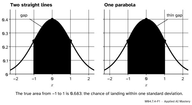
The same three samples, two ways. Two chords (left) cut off the top of the bell and give 0.641. One parabola (right) bends with it and gives 0.693. The truth is 0.683.
A straight line cannot bend, so the chords always cut across the curved top of the bell. A parabola can bend, so it hugs the curve. Simpson’s rule fits a parabola through each three neighbouring samples and adds up the areas under the parabolas. Even this crude one-parabola version is four times closer than the chords, and the gap shrinks very fast as the samples get closer.
Build it up
Step 1. One parabola, three samples. Put the middle sample at 0 and its neighbours at \({-h}\) and \(h\), with heights \(y_0\), \(y_1\), \(y_2\). Write the parabola as \({p(x) = Ax^2 + Bx + C}\).
Step 2. Its area. The term \({Bx}\) is odd, so its areas left and right of 0 cancel:
Step 3. Fit the samples.\({p(0) = y_1}\) gives \({C = y_1}\). The other two conditions are \({Ah^2 - Bh + C = y_0}\) and \({Ah^2 + Bh + C = y_2}\). Adding them removes \(B\), and then:
The middle sample counts four times. A quick check: for a constant height \(c\) the formula gives \({\frac{h}{3} \cdot 6c = 2hc}\), the area of the rectangle. The position of the middle point does not matter either: shifting the picture left or right (a substitution, M04.7.1) changes nothing.
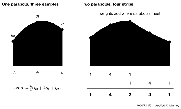
Step 5. Many parabolas. Cut \({[a, b]}\) into an even number \(n\) of strips of width \(h\), and fit one parabola to each pair of strips. Where two parabolas meet, the shared sample collects a weight 1 from each.
M04.7.4-F2
Left: the area under one parabola through three samples is \({\frac{h}{3}(y_0 + 4y_1 + y_2)}\). Right: two parabolas over four strips share the middle sample, so the weights add up to 1, 4, 2, 4, 1.
The formal statement
NoteSimpson’s rule
Let \(n\) be even, \({h = (b - a)/n}\), \({x_k = a + kh}\) and \({y_k = f(x_k)}\). Then \({\int_a^b f(x)\,dx \approx S_n}\), where
The weights run 1, 4, 2, 4, …, 2, 4, 1: 4 at the odd samples, 2 at the even ones inside, and 1 at the two ends.
Exact for cubics. For a quadratic, the parabola through three of its samples is the quadratic itself, so the rule is exact. For \({x^3}\) on \({[-h, h]}\) the true area is 0, because \({x^3}\) is odd, and the rule also gives \({\frac{h}{3}\big((-h)^3 + 4 \cdot 0 + h^3\big) = 0}\). On any double strip, a cubic is a quadratic plus a multiple of \({(x - m)^3}\), where \(m\) is the middle sample; the rule is exact for each part, and both the rule and the integral respect sums and multiples, so the rule is exact for every cubic. That is one degree more than the parabolas were built for, a free gift of symmetry.
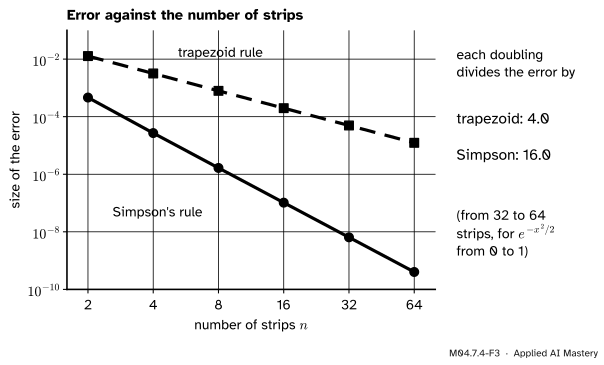
How fast the error falls. For a function with four continuous derivatives, the error of \(S_n\) is at most \({M(b - a)^5/(180\,n^4)}\), where \(M\) bounds \({\abs{f''''}}\) on \({[a, b]}\). The trapezoid rule’s error is at most \({M_2 (b - a)^3/(12\,n^2)}\), with \(M_2\) bounding \({\abs{f''}}\). These bounds are stated here without proof; the box below shows where the powers come from. Their message is in the powers of \(n\): doubling the strips divides the first bound by \({2^4 = 16}\) and the second by \({2^2 = 4}\). The errors themselves behave the same way, as the figure shows for \({\int_0^1 e^{-x^2/2}\,dx}\).
M04.7.4-F3
Error against the number of strips for \({\int_0^1 e^{-x^2/2}\,dx}\), on logarithmic scales. Each doubling divides the trapezoid error by 4 and Simpson’s error by 16, so the two lines have slopes in the ratio 1 to 2.
Go deeper: where the 16 comes from
On one double strip \({[-h, h]}\), Simpson’s rule is exact for everything up to \({x^3}\), so the first thing it can get wrong is \({x^4}\). There the true area is \({2h^5/5}\) and the rule gives \({\frac{h}{3}(h^4 + 0 + h^4) = 2h^5/3}\), an error of \({\frac{2}{3}h^5 - \frac25 h^5 = \frac{4}{15}h^5}\). On a short enough stretch a smooth curve is a cubic plus a small multiple of \({(x - m)^4}\) (the Taylor polynomials of M04.8 make this precise), so each double strip contributes an error of order \(h^5\). There are \({n/2}\) double strips, and \({n = (b - a)/h}\), so the total error is of order \({n h^5 \propto h^4}\). Halve \(h\) and the error shrinks by \({2^4 = 16}\). The same reasoning for the trapezoid rule, which is exact only up to straight lines, gives an error of order \(h^2\), and a factor of 4.
Worked example
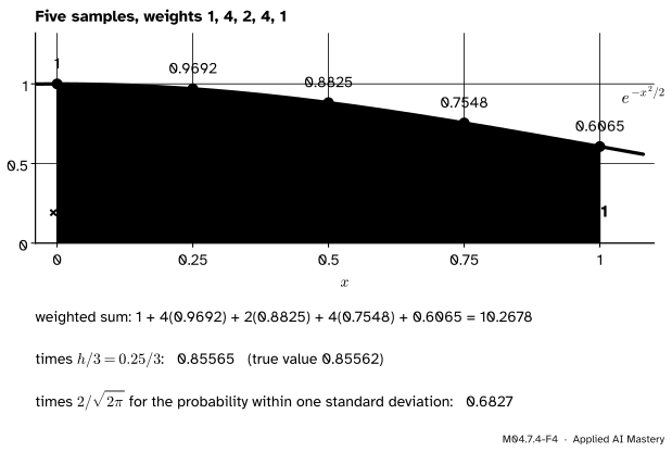
Simpson’s rule by hand for \({\int_0^1 e^{-x^2/2}\,dx}\), with \({n = 4}\). The strip width is \({h = 0.25}\). Sample the bell curve at the five points and weight them 1, 4, 2, 4, 1.
M04.7.4-F4
The worked example as a trace: five samples, their weights, the weighted sum, the factor \({h/3}\), and the step from the area to the probability.
\(x\)
sample
weight
product
0
1
1
1
0.25
0.9692
4
3.8769
0.5
0.8825
2
1.7650
0.75
0.7548
4
3.0194
1
0.6065
1
0.6065
The samples are \({e^{-x^2/2}}\) to four places. The products add up to 10.2678, so
The true value is 0.85562, so the error is about \({2.7 \times 10^{-5}}\). With \({n = 2}\) (samples at 0, 0.5, 1 only) Simpson’s rule gives 0.85609, an error of \({4.6 \times 10^{-4}}\): doubling the strips cut the error by about 17 here, and by closer to 16 as \(n\) grows. The trapezoid rule with the same five samples gives 0.85246, an error of \({-3.2 \times 10^{-3}}\), more than a hundred times worse.
Finally the probability. Let \(X\) have the normal density \(\varphi\). The bell curve is symmetric, so the area from \({-1}\) to 1 is twice the area from 0 to 1, and \(\varphi\) carries the factor \({1/\sqrt{2\pi}}\):
Five samples and a pencil give the 68% rule to four decimal places.
Code
Simpson’s rule from scratch, tested on a cubic (exact) and on \({x^4}\) (not exact), then the error table for the bell curve.
import mathdef simpson(f, a, b, n):"""Composite Simpson's rule with an even number n of strips."""if n %2:raiseValueError("Simpson's rule needs an even number of strips") h = (b - a) / n y = [f(a + k * h) for k inrange(n +1)]return h /3* (y[0] +4*sum(y[1:n:2]) +2*sum(y[2:n -1:2]) + y[n])def trapezoid(f, a, b, n): h = (b - a) / n y = [f(a + k * h) for k inrange(n +1)]return h * (y[0] /2+sum(y[1:n]) + y[n] /2)print("cubic 2x^3 - x^2 + 5 on [0, 2]:", simpson(lambda x: 2* x**3- x**2+5, 0, 2, 2), " exact", 8-8/3+10)print("x^4 on [0, 2]: ", simpson(lambda x: x**4, 0, 2, 2), " exact", 32/5)bell =lambda x: math.exp(-x**2/2)exact = math.sqrt(2* math.pi) *0.5* math.erf(1/ math.sqrt(2)) # the area from 0 to 1, see below# Errors of each rule, and the factor by which each error fell when n doubled.print(f"\n{'n':>2}{'trapez.':>8}{'÷':>4}{'Simpson':>8}{'÷':>4}")previous =Nonefor n in (2, 4, 8, 16, 32, 64): et = trapezoid(bell, 0, 1, n) - exact es = simpson(bell, 0, 1, n) - exact rt =f"{previous[0] / et:4.1f}"if previous else" -" rs =f"{previous[1] / es:4.1f}"if previous else" -"print(f"{n:2d}{et:+.1e}{rt}{es:+.1e}{rs}") previous = (et, es)
The ratios settle on 4 and 16. The exact value used above came from math.erf, Python’s error function, which is the bell curve’s area function under another name: the probability below \(x\) is \({(1 + \operatorname{erf}(x/\sqrt{2}))/2}\). Now the library routines. scipy.integrate.simpson takes samples, so it also works on measured data; scipy.integrate.quad takes the function itself, chooses its own sample points, and returns the value with an estimate of its error.
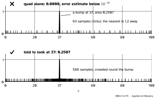
Three methods, one answer: 0.683, 0.954 and 0.997. Last, a warning about trusting the error estimate. quad’s estimate is judged from the samples it took, so a feature that falls between its samples is invisible to the value and to the estimate alike.
bump =lambda x: math.exp(-(x -37)**2/ (2*0.1**2)) # a bell with standard deviation 0.1, centred at 37true_area =0.1* math.sqrt(2* math.pi)alone = integrate.quad(bump, 0, 100)told = integrate.quad(bump, 0, 100, points=[37])print(f"quad alone: {alone[0]:.6f} error estimate {alone[1]:.0e}")print(f"quad told about 37: {told[0]:.6f} error estimate {told[1]:.0e} true {true_area:.6f}")
On its own, quad reports an area of essentially zero with a tiny error estimate, and both are wrong. The argument points tells it where the difficulty lies, and then it finds 0.2507.
Explore
This module’s interactive, the substitution viewer, lives in lesson M04.7.1. It is worth a second look with this lesson in mind. Choose \({x\,e^{-x^2/2}}\): the factor \(x\) is exactly what lets \({u = x^2/2}\) turn the integral into \({\int e^{-u}\,du}\). Without that factor nothing in the \(u\)-panel could absorb \(du\), which is why the plain bell curve has to be sampled instead.
Pitfalls
M04.7.4-F5
Wrong beside right. On its own (top), quad never samples near the narrow bump and reports 0 with a tiny error estimate. Told where to look (bottom), it crowds its samples round the bump and finds 0.2507.
“No antiderivative means the integral does not exist.”
The bell curve is continuous, so its area function exists by the fundamental theorem; it is the normal distribution’s cumulative curve, and libraries evaluate it to full precision. What does not exist is a formula for it in elementary functions. “No formula” and “no answer” are different things.
“Simpson’s rule works with any number of strips.”
The parabolas come in pairs of strips, so \(n\) must be even; the function above refuses an odd \(n\) rather than give a wrong answer. scipy.integrate.simpson accepts any number of samples, but it promises exactness for cubics only for an odd number of equally spaced samples, that is, an even number of strips.
“quad reports its error, so the answer is guaranteed.”
The error estimate is computed from the same samples as the value. The bump above is about 0.4 wide on a range of 100, and quad’s samples step right over it. SciPy’s documentation warns that sharp features may not be integrated correctly. If you know where the action is, pass it in points or split the range, and check against a second method when it matters.
Frontier note: a bell-curve area inside a neural network
The GELU activation of Hendrycks and Gimpel multiplies its input by \({\Phi(x)}\), the probability that a standard normal value lies below \(x\): \({\operatorname{GELU}(x) = x\,\Phi(x)}\). So every forward pass through such a network evaluates bell-curve areas that no elementary formula can give. In code, \({\Phi(x) = (1 + \operatorname{erf}(x/\sqrt{2}))/2}\), the recipe given in the documentation of Python’s math.erf.
Check yourself
Recall
1. Why must areas under the bell curve be computed numerically?
Show answer
\({e^{-x^2/2}}\) has no antiderivative built from elementary functions. The area function exists, but it has no formula of that kind.
2. What is the area under the parabola through three equally spaced samples \({y_0, y_1, y_2}\) with spacing \(h\)?
Show answer
\({\frac{h}{3}(y_0 + 4y_1 + y_2)}\).
3. For which polynomials is Simpson’s rule exact?
Show answer
For every polynomial of degree 3 or less: by construction for quadratics, and for cubics by symmetry.
4. When the number of strips doubles, by about how much do the errors of the trapezoid rule and of Simpson’s rule fall?
Show answer
By about 4 for the trapezoid rule and about 16 for Simpson’s rule.
5. What does quad return besides the value, and why can it mislead?
Show answer
An estimate of the absolute error. It is judged from the same samples as the value, so a narrow feature between the samples fools both.
Exercises
1.★ Apply Simpson’s rule with \({n = 2}\) to \({\int_0^2 x^3\,dx}\) and to \({\int_0^2 x^4\,dx}\), and compare with the exact values.
Show solution
Here \({h = 1}\) and the samples are at 0, 1, 2. For \(x^3\): \({\frac13(0 + 4 \cdot 1 + 8) = 4}\), and the exact value is \({2^4/4 = 4}\): exact, as promised for a cubic. For \(x^4\): \({\frac13(0 + 4 \cdot 1 + 16) = \frac{20}{3} \approx 6.667}\), against the exact \({2^5/5 = 6.4}\). The error is \({\frac{20}{3} - \frac{32}{5} = \frac{4}{15}}\), which is the \({\frac{4}{15}h^5}\) of the box “where the 16 comes from”, with \({h = 1}\).
2.★★ Estimate \({\int_1^2 \frac{dx}{x}}\) with Simpson’s rule and with the trapezoid rule, both with \({n = 4}\), and compare with \({\ln 2}\).
Show solution
With \({h = 0.25}\), the samples at 1, 1.25, 1.5, 1.75, 2 are 1, 0.8, 0.666667, 0.571429, 0.5. Weighted 1, 4, 2, 4, 1 they become 1, 3.2, 1.333333, 2.285714 and 0.5, which add up to 8.319048:
The trapezoid rule halves the two end samples and adds: \({0.25 \times 2.788095 = 0.697024}\). Against \({\ln 2 = 0.693147}\), Simpson’s error is about \({1.1 \times 10^{-4}}\) and the trapezoid error about \({3.9 \times 10^{-3}}\), some 36 times larger.
3.★★★ On one double strip \({[-h, h]}\), let \({M = 2h\,y_1}\) be the midpoint rule and \({T = h(y_0 + y_2)}\) the trapezoid rule with a single strip of width \({2h}\). Show that Simpson’s area is \({(2M + T)/3}\), and check it on \({x^2}\) from 0 to 1.
which is Simpson’s area. For \({x^2}\) on \({[0, 1]}\): \({M = 1 \times 0.5^2 = 0.25}\) and \({T = 1 \times (0 + 1)/2 = 0.5}\), so \({(2M + T)/3 = 1/3}\), the exact area. The midpoint rule errs by about half as much as the trapezoid rule and in the opposite direction, so this weighted average cancels their leading errors, which is how Active Calculus first meets Simpson’s rule.
Summary card
No formula? Sample the curve and fit parabolas: Simpson’s rule is exact for cubics and gains a factor of 16 per doubling.
M04.7.4-F1
Chords cut corners; parabolas bend.
One parabola. Area \({\frac{h}{3}(y_0 + 4y_1 + y_2)}\).
Composite rule. Weights 1, 4, 2, 4, …, 4, 1, times \({h/3}\), with \(n\) even.
Accuracy. Exact for cubics; error \({\propto h^4}\), so ÷16 per doubling (trapezoid: ÷4).
Normal probabilities. 0.683, 0.954, 0.997 within 1, 2, 3 standard deviations.
Sources and next steps
Sources. Each was opened and checked against this lesson on 12 November 2026.
Gilbert Strang and Edwin Herman, Calculus Volume 2 (OpenStax), Section 3.6, Numerical integration: Simpson’s rule built from quadratics through three points (Theorem 3.6, Equation 3.14, with \(n\) even), the error bounds for the midpoint and trapezoid rules (Theorem 3.5) and for Simpson’s rule (Equation 3.15), and Example 3.45, where the bound shows that Simpson’s rule is exact for \({x^3}\). Section 6.4, Working with Taylor series: the subsection on nonelementary integrals states that the antiderivative of \({e^{-x^2}}\) is not an elementary function, and Example 6.23 computes a normal probability with \({e^{-x^2/2}}\).
Matthew Boelkins, Active Calculus (single variable), Section 5.6, Numerical integration: numerical methods motivated by \({\int_0^1 e^{-x^2}\,dx}\), which has no elementary antiderivative, and Simpson’s rule introduced as \({S_{2n} = (2M_n + T_n)/3}\) (Subsection 5.6.4).
David Jerison, MIT OpenCourseWare 18.01SC, Session 63, Numerical integration: the notes of the clip Simpson’s rule fit parabolas to pairs of strips, give the area \({(2\Delta x)(y_0 + 4y_1 + y_2)/6}\), and add the patterns 1 4 1 into 1 4 2 4 1.
SciPy reference, scipy.integrate.quad: the returned error is “an estimate of the absolute error”, points marks places where the integrand is difficult, and sharp features may not be integrated correctly. scipy.integrate.simpson: integrates samples by the composite Simpson’s rule, exactly for polynomials of degree 3 or less when the odd number of samples is equally spaced.
Python documentation, math.erf: the cumulative standard normal distribution written as \({(1 + \operatorname{erf}(x/\sqrt{2}))/2}\).
Dan Hendrycks and Kevin Gimpel, Gaussian Error Linear Units (GELUs): the activation \({x\,\Phi(x)}\), with \(\Phi\) the standard normal cumulative distribution function.
Next. Module M04.8 approximates functions by polynomials with a known error, which explains error orders like the \({h^4}\) above. Probability densities return in M06.6, and numerical integration in M10.8.