Integrating a rate of change gives the total change: velocity gives displacement, a density gives a probability, a slope gives a change in loss. Differentiating and integrating undo each other up to a constant, exactly and on sampled data with NumPy and SciPy.
Use the net change theorem to turn a rate of change into a total change, for a velocity, a growth rate, a probability density and the slope of a loss.
Explain why differentiating an area function gives back f exactly, while integrating a derivative gives back F only up to its starting value.
Show that numpy.diff undoes numpy.cumsum exactly, rounding aside, and that numpy.gradient undoes scipy.integrate.cumulative_trapezoid only approximately, with an error that shrinks as the samples get closer.
Tell net change from total distance, and compute both for a trip that turns back.
In review. The maths and code on this page are checked by automated tests on every change, but an independent reader has not signed it off yet. Spot a mistake or a confusing step? Tell us.
The question
A speedometer reports speed many times a second, never position. Adding up the speeds gives the distance so far, as the last lessons showed. Now go back the other way and take the slopes of that running total. Do you get the speeds back exactly, and what was lost on the way? The same round trip turns the slope of a loss into its total drop, and a density into a probability.
From the last lesson
1. If \({F' = f}\) on an interval, what are all the antiderivatives of \(f\) there?
Show answer
\({F(x) + C}\), for any constant \(C\): two antiderivatives differ by a constant.
2. Why does the constant \(C\) not change \({F(b) - F(a)}\)?
Show answer
It appears in both terms and cancels: \({(F(b) + C) - (F(a) + C)} = {F(b) - F(a)}\).
Intuition
Rates and amounts come in pairs: speed and position, a growth rate and a population, a density and a probability, the slope of a loss and the loss. Integrating takes you from the rate to the amount; differentiating takes you back.
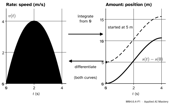
M04.6.4-F1
The round trip for the running trip. Differentiating either position curve gives the same speed. Integrating the speed from 0 gives back only the curve that starts at 0: the starting position, 5 metres for the dashed cart, is lost.
The trip is not symmetric. Going from rate to amount and back, nothing is lost: the slope of the area function is the rate (part one). Going from amount to rate and back, the starting value is lost, because every curve slid up or down has the same slopes.
Build it up
Step 1. A rate integrates to a total change. If \({F'}\) is continuous on \({[a, b]}\), then \(F\) is an antiderivative of \({F'}\), and part two gives
\[
\int_a^b F'(t)\,dt = F(b) - F(a) .
\]
In words: integrating a rate of change gives the total change. This is the net change theorem.
Step 2. Four readings.
Velocity gives displacement.\({\int_a^b v(t)\,dt} = {s(b) - s(a)}\): for the trip over 4 seconds, \({\tfrac{32}{3}}\) metres.
A growth rate gives growth. An app gains users at \({r(t) = 30 + 6t}\) thousand per month (an invented example). Over a year it gains \({\int_0^{12} (30 + 6t)\,dt} = {\big[30t + 3t^2\big]_0^{12}} = 792\) thousand.
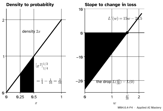
A density gives a probability. If \(X\) has density \({2x}\) on \({[0, 1]}\), the chance that it lands between \({\tfrac14}\) and \({\tfrac12}\) is the area there, \({\big[x^2\big]_{1/4}^{1/2}} = {\tfrac{3}{16}}\) (M06.6).
A slope gives a change in loss. For the running loss, \({L'(w) = 15w - 23.5}\). From \({w = 0}\) to the minimum at \({\tfrac{47}{30}}\) the loss changes by \({\int_0^{47/30} L'(w)\,dw}\), which is \({L(\tfrac{47}{30}) - L(0)} \approx {0.0917 - 18.5} = {-18.41}\): a drop of about 18.41.
M04.6.4-F4
Two more readings of the same theorem. The area under a density between two values is a probability. The area under the slope of a loss is the change in the loss; here it lies below the axis, so the loss falls.
Step 3. Integrate, then differentiate: exact. Start from \(f\), form its area function, and take its slope. Part one says you get \(f\) back:
\[
\frac{d}{dx} \int_a^x f(t)\,dt = f(x) .
\]
Step 4. Differentiate, then integrate: the start is lost. Start from \(F\), take its slope, and integrate from \(a\). The net change theorem with \(x\) as the upper end gives
\[
\int_a^x F'(t)\,dt = F(x) - F(a) ,
\]
which is \(F\) less its starting value. A cart that started 5 metres along has position \({2t^2 - \tfrac13 t^3 + 5}\); its speed is the same \({v(t)}\), and integrating that speed from 0 gives \({2x^2 - \tfrac13 x^3}\). The 5 metres are gone. This is the constant \(C\) again, and it is why a differential equation needs a starting value (M04.9).
Step 5. On samples, sums and differences are exact twins. Data comes as samples, so the integral becomes a running total (numpy.cumsum) and the derivative becomes a difference between neighbours (numpy.diff, which gives \({a_{k+1} - a_k}\)). The same two facts hold with no approximation at all; the formal statement proves them. On a computer only the rounding of decimals can touch the last digits, and whole numbers are not rounded.
Step 6. With trapezoids and slopes, the round trip is close, not exact. The better tools, scipy.integrate.cumulative_trapezoid (the trapezoid rule of M04.5.4 as a running total) and numpy.gradient (central differences, M04.2.4), are not exact inverses. The worked example shows the error, and the code shows it shrinking.
The formal statement
NoteTheorem: net change
If \({F'}\) is continuous on \({[a, b]}\), then
\[
\int_a^b F'(t)\,dt = F(b) - F(a) .
\]
The integral of a rate over an interval is the total change over that interval.
Proof.\(F\) is an antiderivative of the continuous function \({F'}\); apply part two. \(\square\)
The total change is a net change: where the rate is negative, the amount goes down, and that counts against the total. For velocity the net change is the displacement. The total distance counts every metre, forwards or back, so it integrates the speed \({\abs{v(t)}}\) instead.
The round trips, on samples. Let \({x_1, \dots, x_n}\) be numbers, and write \({S_k = x_1 + \dots + x_k}\) for their running totals, with \({S_0 = 0}\).
Total, then difference: exact. Each total is the one before plus one more term, so
\[
S_k - S_{k-1} = x_k .
\]
The differences of the running totals are the numbers you started with. In NumPy, np.diff(np.cumsum(x), prepend=0) gives back x: exactly for whole numbers, and for decimals up to rounding in the last digits, because each running total is rounded as it is stored. Without prepend=0, the first entry is missing.
Difference, then total: the start is lost. Let \({s_0, s_1, \dots, s_n}\) be values and add up their differences. Every inner value appears once with a plus sign and once with a minus sign, so the sum telescopes:
So np.cumsum(np.diff(s)) gives s[1:] - s[0], again up to rounding for decimals: the values less the starting one, the discrete twin of \({F(x) - F(a)}\).
Worked example
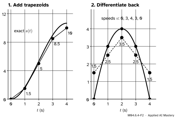
The round trip on the trip’s five samples, by hand. The speeds at \({t = 0, 1, 2, 3, 4}\) seconds are 0, 3, 4, 3, 0 metres per second, one second apart.
Integrate with trapezoids. Each one-second strip becomes a trapezoid of area equal to the average of its two end speeds: 1.5, 3.5, 3.5 and 1.5 metres. The running totals are
\[
0,\; 1.5,\; 5,\; 8.5,\; 10 ,
\]
against the true distances 0, 1.67, 5.33, 9, 10.67 metres. The total, 10 against \({\tfrac{32}{3}}\), is the trapezoid rule’s answer from M04.5.4.
Differentiate back with np.gradient. Inside, it takes the central difference over two seconds; at each end, the one-sided difference over one:
The round trip on samples one second apart. Left: trapezoid running totals trail the true distance. Right: their slopes, by np.gradient, come back as 1.5, 2.5, 3.5, 2.5, 1.5 instead of 0, 3, 4, 3, 0: a blurred copy of the speeds.
The speeds come back blurred. To see why, write out the central difference at an inside sample \({t_k}\), where each trapezoid has area \({\tfrac12 (v_{k-1} + v_k)}\) or \({\tfrac12 (v_k + v_{k+1})}\):
Each recovered speed is a weighted average of the speed and its two neighbours, so the peak of 4 is pulled down to 3.5. When the samples are close, neighbours are nearly equal and the blur fades.
By contrast, plain running totals of the speeds, 0, 3, 7, 10, 10, have differences 3, 4, 3, 0: the speeds again, exactly, less only the first.
Code
First the exact pair, np.cumsum and np.diff: on whole numbers, where nothing is rounded, and then on three decimals.
import numpy as npv = np.array([0, 3, 4, 3, 0]) # the trip's speeds, one second apartS = np.cumsum(v)print("cumsum:", S, " diff of it:", np.diff(S), " with prepend=0:", np.diff(S, prepend=0))s = np.array([5, 8, 12, 15, 15]) # positions of a cart that started at 5print("cumsum of diff:", np.cumsum(np.diff(s)), " s[1:] - s[0]:", s[1:] - s[0])x = np.array([0.1, 0.2, 0.3]) # decimals: each running total is roundedback = np.diff(np.cumsum(x), prepend=0)print("decimals back:", back, f" largest gap from x: {np.max(np.abs(back - x)):.1e}")
cumsum: [ 0  3  7 10 10]   diff of it: [3 4 3 0]   with prepend=0: [0 3 4 3 0]
cumsum of diff: [ 3  7 10 10]   s[1:] - s[0]: [ 3  7 10 10]
decimals back: [0.1 0.2 0.3]   largest gap from x: 5.6e-17
On whole numbers both round trips are exact. On decimals the gap is below \({10^{-16}}\): rounding in the last digits, not an error of the method.
Now the trapezoid pair on the five samples, as in the worked example, and then on samples a hundredth of a second apart. cumulative_trapezoid with initial=0 puts the area up to the first sample, 0, in front, so the result has one entry per sample.
from scipy.integrate import cumulative_trapezoiddef speed(t):return4* t - t **2def position(t):return2* t **2- t **3/3t5 = np.arange(5.0)total5 = cumulative_trapezoid(speed(t5), t5, initial=0)print("trapezoid totals:", total5, " np.gradient:", np.gradient(total5, t5))t = np.linspace(0, 4, 401) # samples 0.01 s aparttotal = cumulative_trapezoid(speed(t), t, initial=0)back = np.gradient(total, t, edge_order=2) # second-order differences at the two ends tooprint(f"largest error in distance: {np.max(np.abs(total - position(t))):.2e} m")print(f"largest error in speed: {np.max(np.abs(back - speed(t))):.2e} m/s")
trapezoid totals: [ 0.   1.5  5.   8.5 10. ]   np.gradient: [1.5 2.5 3.5 2.5 1.5]
largest error in distance: 6.67e-05 m
largest error in speed:    5.00e-05 m/s
With samples a hundredth of a second apart the round trip is good to about \({7 \times 10^{-5}}\) metres and \({5 \times 10^{-5}}\) metres per second. The third exercise shows where the second number comes from: for this speed curve every inside value comes back too low by exactly half the square of the spacing.
Last, each reading of the net change theorem, checked with quad. For the distance, points=[4] tells quad where the speed changes sign, so that it treats the corner of \({\abs{v}}\) carefully.
from scipy.integrate import quadL =lambda w: 7.5* w **2-23.5* w +18.5# the running lossprint(f"users gained: {quad(lambda t: 30+6* t, 0, 12)[0]:.1f} thousand")print(f"probability: {quad(lambda x: 2* x, 0.25, 0.5)[0]:.4f}")print(f"loss change: {quad(lambda w: 15* w -23.5, 0, 47/30)[0]:.4f} L(47/30) - L(0): {L(47/30) - L(0):.4f}")net =round(quad(speed, 0, 6)[0], 4) +0.0# + 0.0 turns a rounded -0.0 into 0.0print(f"0 to 6 s, net: {net:.4f} m distance: {quad(lambda t: abs(speed(t)), 0, 6, points=[4])[0]:.4f} m")
users gained: 792.0 thousand
probability: 0.1875
loss change: -18.4083   L(47/30) - L(0): -18.4083
0 to 6 s, net: 0.0000 m   distance: 21.3333 m
Explore
In the area accumulator of lesson M04.6.2, choose \({\cos t}\) and sweep the end from 0 to \({2\pi}\). The area function climbs to 1, falls to \({-1}\) while the curve is below the axis, and ends where it began: a net change of 0 over a whole turn, although plenty of area was swept.
Pitfalls
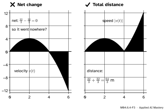
M04.6.4-F3
Wrong beside right, for the trip run on for two more seconds, when the cart rolls back. The velocity integrates to a net change of 0: the cart ends where it started. The distance integrates the speed and counts both legs: \({\tfrac{64}{3} \approx 21.33}\) metres.
“The integral of the velocity is the distance travelled.”
It is the displacement, the net change in position. Run the trip on to 6 seconds: \({\int_0^6 v(t)\,dt = s(6) - s(0) = 0}\), yet the cart went \({\tfrac{32}{3}}\) metres out and \({\tfrac{32}{3}}\) back. For the distance, split at the turning point \({t = 4}\) and add the sizes of the pieces: \({\tfrac{32}{3} + \tfrac{32}{3} = \tfrac{64}{3}}\) metres.
“Integrating undoes differentiating, so I get the function back.”
You get it back less its starting value: \({\int_a^x F'(t)\,dt = F(x) - F(a)}\). From a cart’s speed alone you know how far it moved, not where it is. To know where it is, you also need where it started.
“np.gradient(np.cumsum(v)) gives back v.”
Twice wrong. np.cumsum(v) adds speeds, not areas, so it must be multiplied by the spacing first. And np.gradient takes central differences, which blur the data as the worked example showed. The exact inverse of np.cumsum is np.diff.
Check yourself
Recall
1. State the net change theorem.
Show answer
If \({F'}\) is continuous on \({[a, b]}\), then \({\int_a^b F'(t)\,dt = F(b) - F(a)}\): integrating a rate gives the total change.
2. What does \({\int_a^b v(t)\,dt}\) measure when \(v\) is a velocity?
Show answer
The displacement \({s(b) - s(a)}\), the net change in position. It is the distance travelled only when \(v\) is never negative.
3. What do you get if you differentiate \({\int_a^x f(t)\,dt}\), for a continuous \(f\)?
Show answer
\({f(x)}\), exactly. This is part one of the fundamental theorem.
4. What do you get if you integrate \({F'}\) from \(a\) to \(x\)?
Show answer
\({F(x) - F(a)}\): the function less its starting value, which is lost.
5. Which NumPy function exactly undoes np.cumsum?
Show answer
np.diff, with prepend=0 so that the first entry comes back too. On decimals only rounding in the last digits can differ.
Exercises
1.★ Water runs into a tank at \({r(t) = 6 - t}\) litres per minute for \({0 \le t \le 6}\). How much water enters?
Show solution
The amount is the net change, the integral of the rate:
litres. The rate is never negative, so this is also the total that flowed in.
2.★★ Run the trip on to 5 seconds. Find the cart’s displacement and the distance it travels.
Show solution
The displacement is \({s(5) - s(0)} = {50 - \tfrac{125}{3}} = {\tfrac{25}{3}} \approx 8.33\) metres. The velocity \({4t - t^2}\) is positive before \({t = 4}\) and negative after, so split there. Out: \({s(4) - s(0) = \tfrac{32}{3}}\) metres. Back: \({s(5) - s(4) = \tfrac{25}{3} - \tfrac{32}{3}}\), which is \({-\tfrac73}\), so \({\tfrac73}\) metres. The distance is \({\tfrac{32}{3} + \tfrac73 = 13}\) metres.
3.★★★ Samples of the trip’s speed are a distance \(h\) apart. Show that at an inside sample the trapezoid round trip gives back \({v(t_k) - \tfrac12 h^2}\), exactly.
Show solution
By the worked example, the recovered value is \({\tfrac14 (v_{k-1} + 2v_k + v_{k+1})}\). For \({v(t) = 4t - t^2}\), expanding gives
With \({h = 1}\) the inside values come back 0.5 too low (2.5, 3.5, 2.5), and with \({h = 0.01}\) the error is \({5 \times 10^{-5}}\), as the code found.
Summary card
Integrate a rate to get the change; differentiate the change to get the rate back.
Sources. Each was opened and checked against this lesson on 12 November 2026.
Gilbert Strang and Edwin Herman, Calculus Volume 1 (OpenStax), Section 5.4: Theorem 5.6, the net change theorem \({F(b) = F(a) + \int_a^b F'(x)\,dx}\); net displacement as the integral of the velocity, and total distance as the integral of its absolute value.
Matt Boelkins, Active Calculus, Section 4.4: the total change theorem, the integral of the rate of change of a function is its total change, read for position and velocity as the change in position.
David Jerison, MIT 18.01 Single Variable Calculus (Fall 2006), Lecture 19 notes: the speedometer and the odometer, and a round trip whose net change is 0 while the odometer counts the whole distance.
NumPy documentation (version 2.5): numpy.diff, whose first difference is out[i] = a[i+1] - a[i], and its prepend argument; numpy.gradient, central differences inside and one-sided differences at the boundaries, of first order unless edge_order=2.
SciPy documentation (version 1.18), scipy.integrate.cumulative_trapezoid: the running trapezoid integral, where initial=0 adds a first entry so that the result matches the input in length.
Next. Module M04.7 Integration techniques finds antiderivatives that the table cannot read off directly, and M04.9 meets the lost starting value again as the initial condition of a differential equation.