Why the slope of an area function is the height of the curve: its difference quotient is the average height of a thin strip, squeezed between the strip’s lowest and highest values. So every continuous function has an antiderivative, even the bell curve.
State the first part of the fundamental theorem of calculus, A’(x) = f(x) for a continuous f, and say what each symbol means.
Prove it by trapping a thin strip between the least and greatest values of f on it and applying the squeeze theorem.
Explain why every continuous function has an antiderivative, with the bell curve and the sigmoid as examples.
Differentiate an integral whose upper limit is a function of x, using the chain rule.
Explain why the theorem needs f to be continuous, using the step function and ReLU.
In review. The maths and code on this page are checked by automated tests on every change, but an independent reader has not signed it off yet. Spot a mistake or a confusing step? Tell us.
The question
Transformer networks such as BERT use the GELU activation, \({x\,\Phi(x)}\), where \({\Phi(x)}\) is the area to the left of \(x\) under the standard normal density, a bell curve with total area 1. That area has no formula in the functions you know: it is defined as an area. Yet training the network needs the slope of GELU at every input. How do you differentiate a function that is only defined as an area?
From the last lesson
1. What is the area function of \({f(t) = 5}\) from 0?
Show answer
\({A(x) = 5x}\): the region is a rectangle of height 5 and width \(x\).
2. Where does an area function fall?
Show answer
Where \(f\) is negative, because area below the axis counts as negative and each new strip takes something away.
Intuition
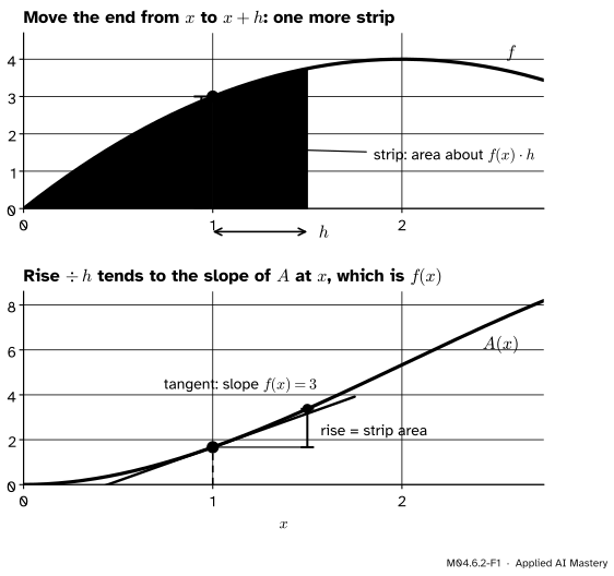
Move the right end from \(x\) to \({x + h}\). The area grows by one thin strip. When the strip is thin, \(f\) hardly changes across it, so the strip is almost a rectangle of height \({f(x)}\) and width \(h\):
\[
A(x + h) - A(x) \;\approx\; f(x)\, h .
\]
M04.6.2-F1
Moving the end on by \(h\) adds one strip under the curve. Top: the strip is nearly a rectangle of height \({f(x)}\). Bottom: the strip’s area is the rise of \(A\) over a run of \(h\), so the rise divided by \(h\) is nearly the slope of the green tangent, \({f(x)}\).
Divide by \(h\) and the left side is the difference quotient of \(A\): the rate at which the area grows. So that rate is about \({f(x)}\). The thinner the strip, the better the “about”, and in the limit the slope of \(A\) at \(x\) is exactly \({f(x)}\). The rest of the lesson makes “about” precise.
Build it up
Step 1. The change is a strip. By the last lesson (Fact 2),
\[
A(x + h) - A(x) = \int_x^{x+h} f(t)\,dt ,
\]
the area of the strip from \(x\) to \({x + h}\).
Step 2. The quotient is an average height. Divide by the width \(h\):
The right side is the average value of \(f\) on the strip (M04.5.3): the height of the rectangle with the same width and the same area.
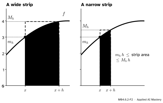
Step 3. Trap the strip. For \({h > 0}\), let \({m_h}\) and \({M_h}\) be the least and the greatest values of \(f\) on the strip. They exist because a continuous function on a closed interval reaches both (the extreme value theorem, M04.4.3). Every height lies between them, so the strip’s area lies between the areas of two rectangles of width \(h\): the short one of height \({m_h}\) and the tall one of height \({M_h}\).
M04.6.2-F2
The strip lies between a short rectangle of height \({m_h}\) and a tall one of height \({M_h}\), the least and the greatest values of \(f\) on it. As the strip narrows, the two heights close in on each other.
Step 4. Divide by \(h\). Dividing the trap by \({h > 0}\) traps the quotient:
Step 5. Shrink the strip.\({m_h}\) and \({M_h}\) are heights of \(f\) at points of the strip. As \(h\) shrinks, those points are squeezed onto \(x\), and because \(f\) is continuous their heights tend to \({f(x)}\). A quantity trapped between two others with the same limit has that limit too: the squeeze theorem (M04.1.2). So the quotient tends to \({f(x)}\).
The formal statement
NoteTheorem: the fundamental theorem of calculus, part one
Let \(f\) be continuous on an interval \(I\) and let \(a\) be a point of \(I\). Then the area function \({A(x) = \int_a^x f(t)\,dt}\) has a derivative at every \(x\) in \(I\), and
\[
\cgrad{A'(x)} = \cdata{f(x)} .
\]
At an end point of \(I\) the derivative is one-sided.
Proof. Fix \(x\) in \(I\). By Step 2 the difference quotient is the average of \(f\) on the strip from \(x\) to \({x + h}\). Take \({h > 0}\) first. With \({m_h}\) and \({M_h}\) the least and greatest values of \(f\) on \({[x, x + h]}\), every \({f(t)}\) there satisfies \({m_h \le f(t) \le M_h}\). The comparison rule (M04.5.3) turns this into \({m_h\, h \le \int_x^{x+h} f(t)\,dt \le M_h\, h}\), and dividing by \({h > 0}\) gives the trap of Step 4.
Now let \(h\) tend to 0. Take any tolerance \({\varepsilon > 0}\). Continuity of \(f\) at \(x\) (M04.1.4) gives a window \({\delta > 0}\) such that \({\abs{f(t) - f(x)} < \varepsilon}\) whenever \({\abs{t - x} < \delta}\). If \({0 < h < \delta}\), every point of the strip is within \(\delta\) of \(x\), so every height on it, the least and the greatest included, is within \(\varepsilon\) of \({f(x)}\):
So for \({0 < h < \delta}\) the quotient is within \(\varepsilon\) of \({f(x)}\). That is the definition of its limit from the right being \({f(x)}\).
For \({h < 0}\) the strip runs from \({x + h}\) to \(x\) and has width \({\abs{h}}\). By the rule for reversed limits, \({A(x + h) - A(x) = -\int_{x+h}^{x} f(t)\,dt}\), and dividing by \({h = -\abs{h}}\) gives
again the average height of a strip next to \(x\). The same trap and the same squeeze show that the limit from the left is \({f(x)}\). The two one-sided limits agree, so \({A'(x) = f(x)}\). \(\square\)
Names. OpenStax calls this part one of the fundamental theorem. MIT’s 18.01 notes and Active Calculus call it the second fundamental theorem. The mathematics is the same.
Every continuous function has an antiderivative. An antiderivative of \(f\) is any function whose derivative is \(f\). Part one hands one over for any continuous \(f\): its area function. That is true even when no formula exists.
The bell curve.\({E(x) = \int_0^x e^{-t^2/2}\,dt}\) has \({E'(x) = e^{-x^2/2}}\). The normal distribution’s cumulative curve is \({\Phi(x) = \tfrac12 + E(x)/\sqrt{2\pi}}\), where \(\tfrac12\) is the area to the left of 0 and \({1/\sqrt{2\pi}}\) makes the total area 1 (M04.7.3, M06.6). So \({\Phi'(x) = e^{-x^2/2}/\sqrt{2\pi}}\), the normal density. The error function, math.erf in Python, is also defined by an area under a bell curve; the code below converts one into the other.
GELU. By the product rule (M04.3.3), the slope of \({x\,\Phi(x)}\) is \({\Phi(x) + x\,\Phi'(x)}\), which at \({x = 1}\) is about \({0.8413 + 0.2420 = 1.0833}\). That answers the question at the top.
The sigmoid. The area function \({S(x) = \int_0^x \sigma(t)\,dt}\) has slope \({\sigma(x)}\). So does softplus, \({\ln(1 + e^x)}\): by the chain rule (M04.3.4) its slope is \({e^x/(1 + e^x)}\), which is \({\sigma(x)}\) after multiplying the top and bottom of \({1/(1 + e^{-x})}\) by \({e^x}\). The code finds \({S(x) - \ln(1 + e^x) = -\ln 2}\) at every \(x\) it tries, and the next lesson proves that two functions with the same slope everywhere differ by a constant. So the area function of the sigmoid is softplus, less \({\ln 2}\).
Upper limits that move. If the upper limit is a function \({g(x)}\), the integral is the area function evaluated at \({g(x)}\): \({G(x) = \int_a^{g(x)} f(t)\,dt = A(g(x))}\). The chain rule and part one give
For example \({\int_0^{x^2} t\,dt}\) has slope \({x^2 \cdot 2x = 2x^3}\). The last lesson’s formula agrees: that integral is \({\tfrac12 (x^2)^2 = \tfrac12 x^4}\), whose slope is \({2x^3}\). A moving lower limit flips the sign: \({\int_x^b f(t)\,dt = A(b) - A(x)}\), whose slope is \({-f(x)}\).
Worked example
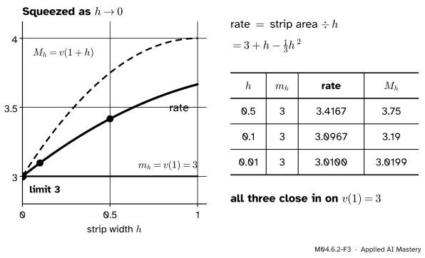
The squeeze, with numbers, for the running trip at \({x = 1}\). The last lesson’s code showed that the trip’s area function from 0 is its position, \({A(x) = 2x^2 - \tfrac13 x^3}\) (lesson M04.6.3 proves it). The strip from 1 to \({1 + h}\) therefore has area
where the first bracket comes from expanding \({2(1 + h)^2 - \tfrac13 (1 + h)^3}\). Dividing by \(h\), the rate is \({3 + h - \tfrac13 h^2}\).
The trap needs the least and greatest speeds on the strip. The speed \({v(t) = 4t - t^2}\) rises until \({t = 2}\), so on \({[1, 1 + h]}\) with \({h \le 1}\) the least is at the left end and the greatest at the right end:
The trap at \({x = 1}\) for the trip. The rate at which the area grows always lies between the least and the greatest speed on the strip, and all three close in on the speed \({v(1) = 3}\).
At \({h = 0.5}\) the trap reads \({3 \le 3.4167 \le 3.75}\); at \({h = 0.1}\), \({3 \le 3.0967 \le 3.19}\). Both bounds tend to 3 as \(h\) tends to 0, so the slope of the area function at 1 is 3 metres per second: the speed at \({t = 1}\), as part one says. The rate \({3 + h - \tfrac13 h^2}\) is the average velocity of M04.2.1, because here the area function is the position.
A moving upper limit. Find the slope of \({G(x) = \int_0^{x^2} e^{-t^2/2}\,dt}\) at \({x = 1}\). With \({g(x) = x^2}\) and \({f(t) = e^{-t^2/2}}\),
No formula for \(G\) was needed; the code checks the number.
Code
From scratch: the area function of the bell curve as a running total of thin strips, then its slope by a central difference (M04.2.4), set beside the height of the curve.
import mathimport numpy as npdef bell(t):return np.exp(-t **2/2)dt =0.0005t = np.linspace(0, 3, 6001) # strip edges from 0 to 3E = np.concatenate([[0.0], np.cumsum(bell(t[:-1] + dt /2) * dt)]) # area from 0 to t[k]for x in (0.0, 0.5, 1.0, 2.0): k, m =round(x / dt), 20# central difference with h = 0.01 lo =max(k - m, 0) # at 0, a one-sided step instead slope = (E[k + m] - E[lo]) / ((k + m - lo) * dt)print(f"x = {x}: slope of E = {slope:.4f} height = {bell(x):.4f}")
x = 0.0: slope of E = 1.0000   height = 1.0000
x = 0.5: slope of E = 0.8825   height = 0.8825
x = 1.0: slope of E = 0.6065   height = 0.6065
x = 2.0: slope of E = 0.1353   height = 0.1353
The library has this area under another name. The error function is \({\operatorname{erf}(z) = \tfrac{2}{\sqrt{\pi}} \int_0^z e^{-u^2}\,du}\), and changing the variable (M04.7) turns that into \({E(x) = \sqrt{\pi/2}\,\operatorname{erf}(x/\sqrt2)}\). The normal cumulative curve follows from it.
for x in (0.5, 1.0, 2.0): by_erf = math.sqrt(math.pi /2) * math.erf(x / math.sqrt(2))print(f"E({x}): strips {E[round(x / dt)]:.6f} erf {by_erf:.6f}")Phi =lambda x: 0.5+0.5* math.erf(x / math.sqrt(2)) # the normal cumulative curvephi =lambda x: math.exp(-x **2/2) / math.sqrt(2* math.pi)gelu_slope = Phi(1) +1* phi(1) # product rule and part oneh =1e-5numeric = ((1+ h) * Phi(1+ h) - (1- h) * Phi(1- h)) / (2* h)print(f"GELU slope at 1: {gelu_slope:.4f} central difference {numeric:.4f}")
central difference: 1.2131
chain rule 2e^(-1/2): 1.2131
Explore
M04.6-X1
Area accumulator
Drag the orange point along the graph, or use the slider, and watch the area function grow in the lower panel. Shrink the strip width \(h\) and compare the strip’s rate with the height \({f(x)}\). Then try \({\cos t}\), where the area falls while the curve is below the axis, and the step, whose area function has a corner.
The read-out gives the area so far, the height, the strip’s area and its rate. For the sigmoid it also shows the area function as softplus less a constant, and for the bell curve its link to the normal cumulative curve.
Pitfalls
M04.6.2-F4
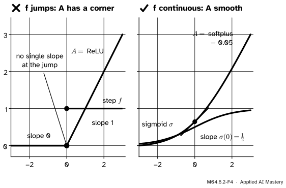
Wrong beside right, with both area functions starting at \({t = -3}\). The step jumps at 0, and its area function, ReLU, has a corner there: slope 0 from the left, 1 from the right. The sigmoid, a step with the jump smoothed out, is continuous, and its area function is smooth with slope \({\sigma(x)}\) everywhere.
“Part one works for any function I can integrate.”
It needs \(f\) to be continuous at \(x\). The step function can be integrated, and its area function from any start left of 0 is ReLU, \({\max(0, x)}\). At 0 the step jumps, and ReLU has no slope there: 0 from the left, 1 from the right. Away from the jump the theorem holds again, which is why ReLU’s slope is the step everywhere except at 0.
“The slope of \({\int_0^{x^2} f(t)\,dt}\) is \({f(x^2)}\).”
The upper limit moves at rate \({2x}\), so the chain rule adds that factor: the slope is \({f(x^2) \cdot 2x}\). Test with \({f(t) = t}\): the integral is \({\tfrac12 x^4}\), whose slope is \({2x^3}\), not \({x^2}\).
“The slope of \({\int_x^5 f(t)\,dt}\) is \({f(x)}\).”
Moving the lower end to the right removes area, so the slope is \({-f(x)}\). Write the integral as \({A(5) - A(x)}\) and differentiate.
Check yourself
Recall
1. State part one of the fundamental theorem of calculus.
Show answer
If \(f\) is continuous on an interval containing \(a\), the area function \({A(x) = \int_a^x f(t)\,dt}\) has derivative \({A'(x) = f(x)}\) at every \(x\) of the interval.
2. What is the difference quotient \({(A(x + h) - A(x))/h}\), in terms of the strip?
Show answer
The average height of \(f\) on the strip between \(x\) and \({x + h}\): the strip’s area divided by its width.
3. Which two numbers trap that quotient, and which theorem pins its limit?
Show answer
The least and the greatest values of \(f\) on the strip, \({m_h}\) and \({M_h}\). Both tend to \({f(x)}\) because \(f\) is continuous, so the squeeze theorem gives the limit \({f(x)}\).
4. What is the slope of \({\int_0^x e^{-t^2/2}\,dt}\) at \({x = 0}\)?
Show answer
\({e^{0} = 1}\), the height of the bell curve at 0.
5. Why has the area function of the step function no slope at 0?
Show answer
The step jumps at 0, so the theorem’s continuity condition fails there. Its area function is ReLU, with slope 0 from the left and 1 from the right.
Exercises
1.★ Find the slope of \({F(x) = \int_1^x \sqrt{1 + t^3}\,dt}\), and its value at \({x = 2}\).
Show solution
The integrand is continuous for \({t \ge -1}\), so part one gives \({F'(x) = \sqrt{1 + x^3}}\) there. At \({x = 2}\), \({F'(2) = \sqrt{1 + 8} = 3}\). No formula for \(F\) is needed.
2.★★ Find the slope of \({H(x) = \int_0^{3x} e^{-t^2/2}\,dt}\), and its value at \({x = 0}\).
Show solution
The upper limit is \({g(x) = 3x}\), with \({g'(x) = 3}\). By the chain rule and part one,
At \({x = 0}\) this is 3: near 0 the bell curve has height about 1, and the upper limit moves three times as fast as \(x\).
3.★★★ Let \({G(x) = \int_x^{x^2} t\,dt}\), where both limits move. Find \({G'(x)}\) with part one, then check it with the area function \({\tfrac12 x^2}\) of the last lesson.
Show solution
With \(A\) the area function of \({f(t) = t}\) from 0, \({G(x) = A(x^2) - A(x)}\). The chain rule on the first term and part one on both give
Check: \({A(x) = \tfrac12 x^2}\), so \({G(x) = \tfrac12 x^4 - \tfrac12 x^2}\), whose slope is \({2x^3 - x}\) by the power rule. The two agree.
Summary card
The slope of the area function is the height of the curve: \({A'(x) = f(x)}\) for continuous \(f\).
M04.6.2-F1
One more strip: rise about \({f(x)\,h}\).
Part one. For continuous \(f\) and \({A(x) = \int_a^x f(t)\,dt}\), \({A'(x) = f(x)}\).
Why. The quotient is the strip’s average height, trapped between \({m_h}\) and \({M_h}\).
So every continuous \(f\) has an antiderivative. The bell curve’s leads to \(\Phi\); the sigmoid’s is softplus less \({\ln 2}\).
Moving limit. The slope of \({\int_a^{g(x)} f(t)\,dt}\) is \({f(g(x))\, g'(x)}\).
Needs continuity. At a jump of \(f\) the area function has a corner.
Sources and next steps
Sources. Each was opened and checked against this lesson on 12 November 2026.
Gilbert Strang and Edwin Herman, Calculus Volume 1 (OpenStax), Section 5.3: Theorem 5.4, part 1 of the fundamental theorem, for \(f\) continuous on \({[a, b]}\). Its proof writes the difference quotient as the average of \(f\) on \({[x, x + h]}\) and uses the mean value theorem for integrals (Theorem 5.3), whose own proof traps \(f\) between its least and greatest values.
David Jerison, MIT 18.01 Single Variable Calculus (Fall 2006), Lecture 20 notes: the second fundamental theorem, \({F'(x) = f(x)}\) for \({F(x) = \int_a^x f(t)\,dt}\) with \(f\) continuous; the strip proof \({\Delta F \approx f(x)\,\Delta x}\) and the average-value proof; and the error function as a new function defined by an integral.
Matt Boelkins, Active Calculus, Section 5.2: the same theorem under the name second fundamental theorem, and the integral function \({\int_0^x e^{-t^2}\,dt}\), which it notes has no elementary antiderivative.
Ian Goodfellow, Yoshua Bengio and Aaron Courville, Deep Learning, Section 3.10: softplus \({\zeta(x) = \log(1 + \exp(x))}\), its derivative \({\sigma(x)}\) (equation 3.37), and \({\zeta(x) = \int_{-\infty}^x \sigma(y)\,dy}\) (equation 3.40).
Dan Hendrycks and Kevin Gimpel, Gaussian Error Linear Units (GELUs), 2016: the GELU activation is \({x\,\Phi(x)}\), with \(\Phi\) the standard Gaussian cumulative distribution function.