Join neighbouring samples with straight lines and the rectangles become trapezoids: the average of the left and right sums, and far more accurate. The rule needs only samples, so it integrates tables of data, from a cart’s speedometer readings to the points of an ROC curve.
Derive the area of one trapezoid and the trapezoid rule, with weights of one half at the ends, and show that it is the average of the left and right sums.
Apply the trapezoid rule by hand to a function and to a table of samples, with equal or unequal spacing.
Show that the trapezoid error for x^2 on [0, 1] is exactly 1/(6n^2), and observe in a table that doubling the strips cuts the error by about four, against about two for the left sum.
Compute the area under an ROC curve with the trapezoid rule, from scratch and with scipy.integrate.trapezoid, passing the arguments in the right order.
In review. The maths and code on this page are checked by automated tests on every change, but an independent reader has not signed it off yet. Spot a mistake or a confusing step? Tell us.
The question
Most data never arrives as a formula. A speedometer is read once a second, a sensor logs a temperature once a minute, and an ROC curve comes as a list of points. You have samples, not a function, and you still want the area under them. What area do the samples give, and how good is it? When a library such as scikit-learn reports an “area under the curve” from a list of points, it uses the rule of this lesson.
From the last lesson
1. For a velocity \(v\), what do \({\int_a^b v\,dt}\) and \({\int_a^b \abs{v}\,dt}\) measure?
Show answer
The net distance, which is the change in position, and the distance travelled.
2. What is the average value of the cart’s speed over its first 4 seconds?
Show answer
The integral divided by the length: \({(32/3)/4 = 8/3 \approx 2.67}\) m/s.
Intuition
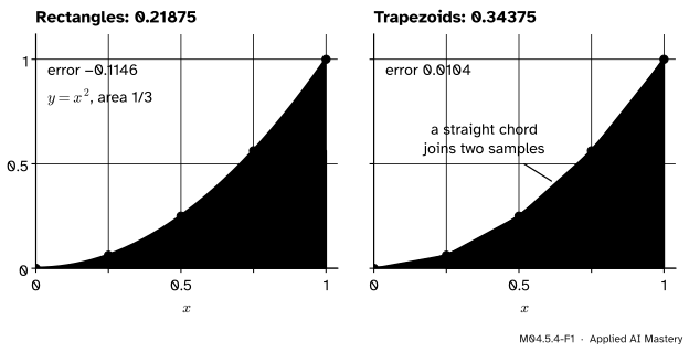
A left or a right sum gives each strip a flat top at the height of one of its ends. Yet we know the height at both ends. Join the two sample points with a straight line and the strip becomes a trapezoid, whose slanted top follows the curve far more closely than a flat one.
M04.5.4-F1
The same five samples, two ways to fill the strips. Flat tops leave large errors; straight chords between neighbouring samples leave only thin slivers, and the error drops from 0.1146 to 0.0104.
Build it up
Write \({y_k = f(x_k)}\) for the sample at the cut point \(x_k\), with \({k = 0, 1, \dots, n}\).
Step 1. One trapezoid. The strip from \(x_{k-1}\) to \(x_k\) has width \({\Delta x}\) and sides of height \(y_{k-1}\) and \(y_k\). Cut it into a rectangle of height \(y_{k-1}\) and a triangle of base \({\Delta x}\) and height \({y_k - y_{k-1}}\). Its area is
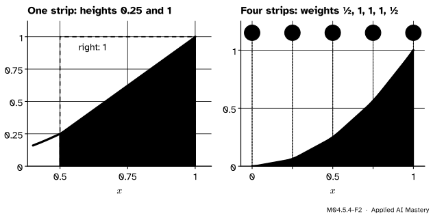
If the right side is the shorter one, cut off a rectangle of height \(y_k\) instead, with a triangle of height \({y_{k-1} - y_k}\) on it; the same steps give the same result. So a trapezoid’s area is its width times the average of its two heights. That is also the average of the left rectangle, \({\Delta x\,y_{k-1}}\), and the right rectangle, \({\Delta x\,y_k}\).
Step 2. Add the \(n\) trapezoids. In the sum, each inside height \(y_1\) to \(y_{n-1}\) is a side of two trapezoids, so it is counted twice with a half; each end height is a side of only one:
Left: a trapezoid’s area is the strip width times the average of its two heights, halfway between the left and the right rectangle. Right: every inside height is a side of two trapezoids, so the weights are ½ at the ends and 1 inside.
Step 3. The average of the two sums. Add the left and right sums. The left sum uses \(y_0\) to \(y_{n-1}\) and the right sum \(y_1\) to \(y_n\), so the inside heights appear in both:
So \({\text{Trap}(n) = (\text{Left}(n) + \text{Right}(n))/2}\).
Step 4. Four strips of \({x^2}\). The left and right sums were 0.21875 and 0.46875, so \({\text{Trap}(4) = 0.34375}\). The error, \({0.34375 - 1/3 = 1/96 \approx 0.0104}\), is eleven times smaller than the left sum’s error of 0.1146.
The formal statement
NoteDefinition: the trapezoid rule
For \(n\) equal strips of width \({\Delta x = (b - a)/n}\) with samples \({y_k = f(x_k)}\),
\[
\text{Trap}(n) = \sum_{k=1}^{n} \frac{y_{k-1} + y_k}{2}\,\Delta x .
\]
For samples \({(x_0, y_0), \dots, (x_n, y_n)}\) at any spacing, each trapezoid has its own width:
The rule uses nothing but the samples. It never needs a formula for \(f\), which is why it can integrate a table of measurements.
The error for \({x^2}\) on \({[0, 1]}\), exactly. Lesson M04.5.2 found \({\text{Right}(n) = \tfrac13 + \tfrac{1}{2n} + \tfrac{1}{6n^2}}\), and the gap between the right and left sums is \({1/n}\). The average of the two sums sits halfway down the gap, so
The trapezoid error is exactly \({1/(6n^2)}\). With twice as many strips it is divided by exactly 4. The left and right errors are close to \({1/(2n)}\) in size, and twice as many strips only about halves them. In the left and right sums the big terms \({\tfrac{1}{2n}}\) have opposite signs, and averaging cancels them.
Which way it errs. A chord between two points of a curve that bends upwards, like \({x^2}\), lies above the curve, so the trapezoid rule overestimates. A chord of a curve that bends downwards, like the cart’s speed, lies below it, so the rule underestimates.
Go deeper: how big can the trapezoid error be?
For a function whose second derivative never exceeds \(M\) in size on \({[a, b]}\), the error of the trapezoid rule is at most
\[
\frac{M\,(b - a)^3}{12\,n^2} .
\]
This bound is stated here without proof. For \({x^2}\) on \({[0, 1]}\), \({f'' = 2}\) gives \({1/(6n^2)}\): the bound is reached exactly. The \({n^2}\) in the bottom is why, for a typical smooth function, the error falls by about four each time \(n\) doubles. (It can fall faster: for some functions the errors on different strips cancel even better.)
Worked example
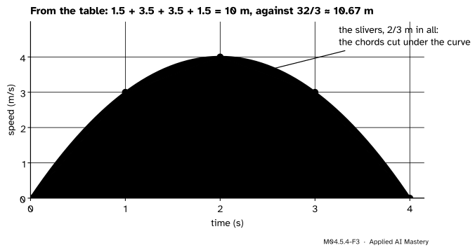
The cart’s distance from its table. The speeds are 0, 3, 4, 3 and 0 m/s at \({t = 0, 1, 2, 3, 4}\) s, so \({\Delta t = 1}\) and the weights alone multiply the readings:
Four trapezoids from the five readings, each its width times its average height. The speed curve bends down, so every chord cuts under it and the total falls short by the slivers.
The true distance is 32/3 ≈ 10.67 m, so the error is \({10 - 32/3 = -2/3}\) m. The rule underestimates, as it must for a curve that bends down.
Twice as many readings. At half-second intervals the speeds are 0, 1.75, 3, 3.75, 4, 3.75, 3, 1.75 and 0. Both ends are 0, so
The error is now \({10.5 - 32/3 = -1/6}\) m, a quarter of \({-2/3}\): doubling the readings divided the error by 4.
An ROC curve. The ten students of ML01.7.3 give an ROC curve, with the false positive rate across and the true positive rate up, through (0, 0), (0, 0.4), (0.2, 0.4), (0.2, 0.8), (0.6, 0.8), (0.6, 1) and (1, 1). The spacing is uneven. Three of the widths are 0 and add nothing; on each of the other three steps the two heights are equal, so the average height is just that height:
That is the AUC of 0.80 that ML01.7.3 found by counting pairs.
Code
From scratch, the rule for samples at any spacing is a loop over neighbouring pairs.
def trapezoid_rule(y, x):"""Area under the samples (x[k], y[k]), joined by straight lines.""" total =0.0for k inrange(1, len(x)): total = total + (x[k] - x[k -1]) * (y[k -1] + y[k]) /2return totalt = [0, 1, 2, 3, 4]speeds = [0, 3, 4, 3, 0]t_half = [k /2for k inrange(9)]speeds_half = [4* s - s **2for s in t_half]fpr = [0, 0, 0.2, 0.2, 0.6, 0.6, 1.0]tpr = [0, 0.4, 0.4, 0.8, 0.8, 1.0, 1.0]print("trip, one-second readings: ", trapezoid_rule(speeds, t))print("trip, half-second readings:", trapezoid_rule(speeds_half, t_half))print("area under the ROC curve: ", round(trapezoid_rule(tpr, fpr), 4))
trip, one-second readings:  10.0
trip, half-second readings: 10.5
area under the ROC curve:   0.8
Now two tables that show the factor of four. The bell curve \({e^{-x^2/2}}\) has no antiderivative that can be written with the usual functions (M04.7.4), so the reference value comes from scipy.integrate.quad, a precise library integrator.
import numpy as npfrom scipy.integrate import quaddef left_sum(f, a, b, n): dx = (b - a) / nreturn np.sum(f(a + np.arange(n) * dx)) * dxdef trap(f, a, b, n): y = f(np.linspace(a, b, n +1))return (b - a) / n * (y[0] /2+ y[1:-1].sum() + y[-1] /2)bell =lambda x: np.exp(-x **2/2)exact, _ = quad(bell, 0, 2)print(f"exact area, 0 to 2: {exact:.6f}")errors = {} # n: (left-sum error, trapezoid error)for n in [4, 8, 16, 32, 64]: errors[n] = (left_sum(bell, 0, 2, n) - exact, trap(bell, 0, 2, n) - exact)for j, rule, places in [(0, "left sum", 6), (1, "trapezoids", 7)]:print(f"\n{rule}\n n error ratio")for n, e in errors.items(): ratio =f"{errors[n //2][j] / e[j]:.2f}"if n >4else""print(f"{n:4d}{e[j]:10.{places}f}{ratio}")
exact area, 0 to 2: 1.196288

left sum
   n       error  ratio
   4    0.210552
   8    0.106675  1.97
  16    0.053689  1.99
  32    0.026933  1.99
  64    0.013488  2.00

trapezoids
   n       error  ratio
   4  -0.0056142
   8  -0.0014083  3.99
  16  -0.0003523  4.00
  32  -0.0000881  4.00
  64  -0.0000220  4.00
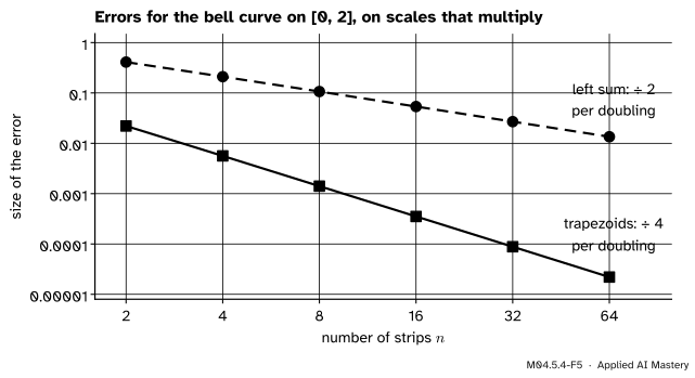
Each doubling of \(n\) about halves the left-sum error and divides the trapezoid error by very nearly four. The figure draws both tables on scales where each step multiplies by a fixed factor.
M04.5.4-F5
The errors of the two tables, with \({n = 2}\) added, for the bell curve on \({[0, 2]}\). On these scales each rule’s errors lie on a straight line, and the trapezoid line is twice as steep.
Finally the library. SciPy’s trapezoid(y, x) takes the heights first and the positions second, or a spacing dx when the samples are evenly spaced. scikit-learn’s auc(x, y) runs the same rule with the positions first.
This module’s interactive, the Riemann refiner, lives in lesson M04.5.2. Choose the trapezoid rule and press Double the strips: the read-out shows the error falling by about four each time. Switch to the left rule on the same function and watch the factor drop to about two.
Pitfalls
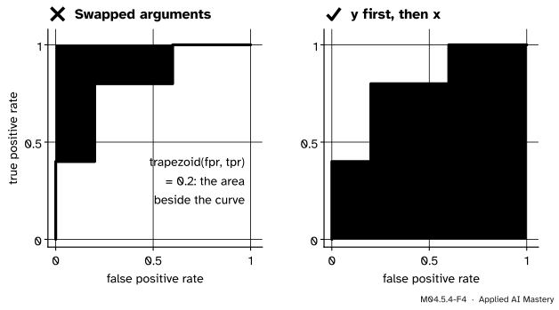
M04.5.4-F4
Wrong beside right. With its arguments swapped, the trapezoid rule integrates sideways and measures the area between the curve and the vertical axis, 0.2, instead of the area under it, 0.8.
“trapezoid(fpr, tpr) is the area under the ROC curve.”
SciPy’s order is trapezoid(y, x): heights first. Swapped, it measures the area beside the curve, which for an ROC curve is 1 minus the AUC, here 0.2. scikit-learn’s auc(x, y) takes the positions first, the other way round, so check each library’s order rather than guess.
“The samples are enough; the spacing takes care of itself.”
Given only y, scipy.integrate.trapezoid assumes the samples are 1 apart. For the half-second readings trapezoid(speeds_half) returns 21, twice the 10.5 it should give. Pass the positions, or dx=0.5.
“The trapezoid rule always overestimates.”
It overestimates for \({x^2}\), whose chords lie above the curve, and underestimates for the cart’s speed, whose chords lie below it: 0.34375 against 1/3, but 10 against 32/3. The sign of the error follows the way the curve bends.
Check yourself
Recall
1. What is the area of one trapezoid of width \({\Delta x}\) with sides \(y_0\) and \(y_1\)?
Show answer
\({\Delta x\,(y_0 + y_1)/2}\): the width times the average of the two heights.
2. With \(n\) equal strips, what weights do the samples get in the trapezoid rule?
Show answer
\({\tfrac12}\) for the two end samples and 1 for every inside sample, all times \({\Delta x}\).
3. How is \({\text{Trap}(n)}\) related to the left and right sums?
4. When the number of strips doubles, by about how much does the trapezoid error fall, and the left-sum error?
Show answer
The trapezoid error falls by about 4 (exactly 4 for \({x^2}\)), the left-sum error by about 2.
5. In scipy.integrate.trapezoid(y, x), which argument holds the heights, and what spacing is assumed if x is left out?
Show answer
y holds the heights and x the positions. Without x the samples are taken to be dx apart, and dx is 1 unless you give it.
Exercises
1.★ Find the trapezoid rule for \({x^2}\) on \({[0, 1]}\) with two strips in two ways: with the weights, and as the average of the left and right sums. Check the error against \({1/(6n^2)}\).
Show solution
With \({\Delta x = 1/2}\) the samples are 0, 1/4 and 1. With the weights,
As an average, the left and right sums are 1/8 and 5/8, and \({(1/8 + 5/8)/2 = 3/8}\). The error is \({3/8 - 1/3 = 1/24}\), and \({1/(6 \times 2^2) = 1/24}\).
2.★★ Two passes and two fails are scored, and one pass ties with one fail. The ROC curve runs through (0, 0), (0, 0.5), (0.5, 1) and (1, 1); the slanted step comes from the tie. Find its area with the trapezoid rule, and with flat tops at the left height of each step. Which agrees with counting pairs, where a tie counts as half a pair in the right order?
Flat tops at the left heights give \({0.5 \times 0.5 + 0.5 \times 1 = 0.75}\). Counting pairs: the higher pass outranks both fails (2 pairs), and the other pass outranks one fail and ties with the other (1.5 pairs), so 3.5 of the 4 pairs are in order, \({3.5/4 = 0.875}\). The trapezoid rule agrees, because the slanted step gives the tie half credit.
3.★★★ Show that the trapezoid rule with \(n\) equal strips gives exactly \({\tfrac{32}{3}\big(1 - \tfrac{1}{n^2}\big)}\) metres for the cart from 0 to 4 s. What is the smallest \(n\) that makes the error less than 1 cm?
Show solution
The speed is 0 at both ends, so the end samples add nothing and the trapezoid rule equals the left sum. With \({\Delta t = 4/n}\) and \({t_k = 4k/n}\), the speed is \({v(t_k) = 16k/n - 16k^2/n^2}\), so
At \({n = 4}\) this is \({\tfrac{32}{3} \cdot \tfrac{15}{16} = 10}\), as in the worked example. The error is \({32/(3n^2)}\), below 0.01 when \({n^2 > 3200/3 \approx 1066.7}\). Since \({32^2 = 1024}\) and \({33^2 = 1089}\), the smallest \(n\) is 33.
Summary card
Join neighbouring samples with straight lines: the trapezoid rule averages the left and right sums.
M04.5.4-F1
Flat tops against straight chords.
One trapezoid. Width times the average height, \({\Delta x\,(y_{k-1} + y_k)/2}\).
Equal strips. Weights ½, 1, …, 1, ½ times \({\Delta x}\), the average of the left and right sums.
Error. Divided by about 4 when \(n\) doubles; exactly \({1/(6n^2)}\) for \({x^2}\) on \({[0, 1]}\).
Data. Any spacing works: the trip’s table gives 10 m and the ROC curve 0.8.
Sources. Each was opened and checked against this lesson on 12 November 2026.
Gilbert Strang and Edwin Herman, Calculus Volume 2 (OpenStax), Section 3.6, Numerical Integration. It states the trapezoidal rule (Theorem 3.4), writes it as half the sum of the left and right endpoint approximations, and gives the error bound for the midpoint and trapezoidal rules (Theorem 3.5), with the \({(b - a)^3/(12n^2)}\) of the deeper block above.
SciPy reference, scipy.integrate.trapezoid: the signature trapezoid(y, x=None, dx=1.0, axis=-1), and that without x the samples are taken to be evenly spaced dx apart.
scikit-learn reference, sklearn.metrics.auc, which computes the area under a curve “using the trapezoidal rule” and takes the positions x first.
David Jerison, MIT OpenCourseWare 18.01SC, Session 63: Numerical Integration, and its lecture notes, which call Riemann sums a very inefficient way to estimate an area and the trapezoidal rule much more reasonable.
Next. Module M04.6 proves the fundamental theorem of calculus, which turns the area under a curve into a difference of two values of an antiderivative. Lesson M04.7.4 returns to numerical integration with Simpson’s rule, whose error falls by about sixteen when the strips double.