With no formula at hand, a computer estimates a slope from a few function values. Build the forward and central differences, find their errors exactly on x cubed, watch rounding take over at tiny steps, then use numpy.gradient, scipy.differentiate and the gradient check.
Compute forward and central difference estimates of a derivative, by hand and in code.
Derive the errors of both differences on x cubed, 3xh + h^2 and h^2, and predict what halving h does to each.
Explain why the error grows again when h is very small, and choose a sensible step.
Estimate derivatives with numpy.gradient from sampled data and with scipy.differentiate.derivative from a function.
Check a derivative found by hand against a central difference with a relative-error test.
In review. The maths and code on this page are checked by automated tests on every change, but an independent reader has not signed it off yet. Spot a mistake or a confusing step? Tell us.
The question
You have worked out the slope of a loss by hand and written it into your training code. A dropped minus sign or a missing factor of 2 would not crash anything: the model would simply train badly, and you might never learn why. How can a computer tell you, in a few lines, that your slope is right?
From the last lesson
1. What is the derivative of \({1/x}\)?
Show answer
\({-1/x^2}\), for every \({x \neq 0}\).
2. What are ReLU’s one-sided slopes at 0?
Show answer
0 from the left and 1 from the right, so ReLU has no derivative at 0.
Intuition
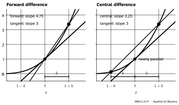
A computer cannot take a limit, but it can evaluate a function at a few points and divide. That is the difference quotient of lesson 1 with a small, fixed step \(h\): a secant slope standing in for the tangent’s. The picture compares two ways to place that secant on \({y = x^3}\) at \({x = 1}\), with a deliberately large step, \({h = 0.5}\), so that the difference shows.
M04.2.4-F1
Two secants with the same step \({h = 0.5}\). Looking one way (left), the slope is 4.75; looking both ways (right), it is 3.25. The true slope is 3.
The forward difference looks one way, from \(x\) to \({x + h}\), and its secant leans well off the tangent: slope 4.75. The central difference looks both ways, from \({x - h}\) to \({x + h}\). The bend of the curve pulls that secant up on one side and down on the other, the two pulls nearly cancel, and it runs almost parallel to the tangent: slope 3.25. Same step, same number of function values, far better answer.
Build it up
Step 1. Forward. The forward difference is lesson 1’s quotient with \(h\) kept small instead of sent to 0. For \({x^3}\) at 1 with \({h = 0.1}\): \({(1.331 - 1)/0.1 = 3.31}\).
Step 2. Backward. Looking left instead, \({(f(x) - f(x - h))/h}\) gives \({(1 - 0.729)/0.1 = 2.71}\). One overshoots the true slope 3 and the other undershoots it.
Step 3. Average them. The mean of 3.31 and 2.71 is 3.01. In symbols, the \({f(x)}\) terms cancel:
which is the slope of the secant through the two points either side of \(x\), the central difference.
Step 4. Compare. With \({h = 0.1}\) the forward difference misses by 0.31 and the central one by 0.01. Each needs two function values, yet one is thirty times closer.
The formal statement
NoteDefinition: forward and central differences
For a small step \({h > 0}\), the forward difference and the central difference of \(f\) at \(x\) are
Letting \(h\) tend to 0 in either line gives the derivative \({3x^2}\), which is 3 at \({x = 1}\). The errors are what remains: \({3xh + h^2}\) against \({h^2}\). Halve \(h\) and the forward error becomes \({3xh/2 + h^2/4}\), about half when \(h\) is small, while the central error becomes exactly a quarter. An error proportional to \(h\) is called first order, one proportional to \({h^2}\)second order. M04.8.4 shows, with Taylor polynomials, that the same orders hold for every smooth function, not just \({x^3}\).
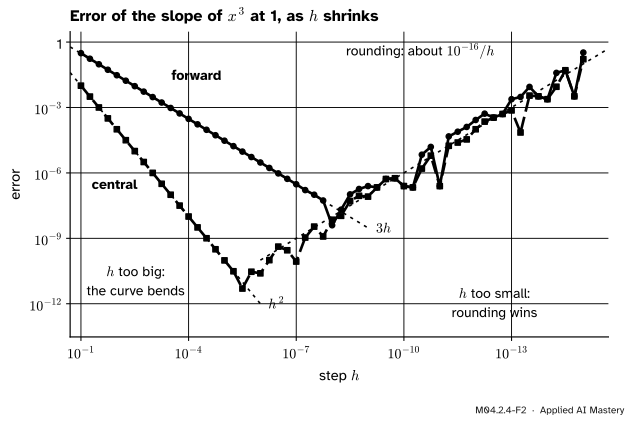
When \(h\) is too small. The algebra says: shrink \(h\), shrink the error. A computer disagrees once \(h\) is tiny. Python stores a number in 53 binary digits, about 16 significant decimal digits, so every computed value, even \({x + h}\) itself, carries a rounding error of about \({10^{-16}}\) times its size: \({1 + 10^{-16}}\) is stored as exactly 1. Subtracting two nearly equal values, \({f(x+h) - f(x)}\), cancels their leading digits but keeps those rounding errors, and dividing by a tiny \(h\) magnifies them to about \({10^{-16}/h}\). So the total error is roughly the truncation error plus \({10^{-16}/h}\): the first falls as \(h\) shrinks and the second rises.
M04.2.4-F2
The error of each difference for \({x^3}\) at 1, as \(h\) shrinks to the right. Truncation error falls like \({3h}\) or \({h^2}\); rounding error rises like \({10^{-16}/h}\). Each difference is best in between.
The forward difference does best near \({h = 10^{-8}}\), where both errors are about \({10^{-8}}\). The central difference, whose truncation error falls faster, does best near \({h = 10^{-5}}\) or \({10^{-6}}\), with an error near \({10^{-11}}\). Below that, smaller steps make things worse, and at \({h = 10^{-15}}\) both estimates are wrong in the first decimal place. The exact digits in that region depend on how each value happens to round; M10.1 and M10.8 treat rounding fully.
Worked example
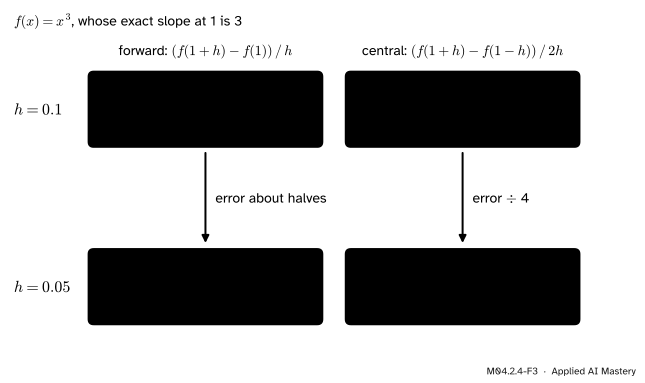
The slope of \({x^3}\) at 1, by hand, with \({h = 0.1}\) and then \({h = 0.05}\). The exact answer is 3.
With \({h = 0.1}\): \({f(1.1) = 1.331}\) and \({f(0.9) = 0.729}\). The forward difference is \({(1.331 - 1)/0.1 = 3.31}\), an error of \({0.31 = 3 \times 0.1 + 0.1^2}\). The central difference is \({(1.331 - 0.729)/0.2 = 3.01}\), an error of \({0.01 = 0.1^2}\).
With \({h = 0.05}\): \({f(1.05) = 1.157625}\) and \({f(0.95) = 0.857375}\). The forward difference is \({0.157625/0.05 = 3.1525}\), an error of 0.1525; the central difference is \({0.30025/0.1 = 3.0025}\), an error of 0.0025.
M04.2.4-F3
The worked example as a trace. Halving the step roughly halves the forward error (0.31 to 0.1525) and exactly quarters the central one (0.01 to 0.0025), as \({3xh + h^2}\) and \({h^2}\) predict.
Sampled data: the cart’s velocity from its positions. First the truth to compare with. The definition, worked as in lesson 1 but at any time \(t\), gives the cart’s velocity at every instant. With \({s(t) = 2t^2 - t^3/3}\), the two parts of \({s(t+h)}\) multiply out to
Subtracting the second from the first, and then \({s(t)}\), leaves \({s(t+h) - s(t)} = {4th} + {2h^2} - {t^2h} - {th^2} - {h^3/3}\). Dividing by \(h\) gives \({4t} - {t^2} + {2h} - {th} - {h^2/3}\), which tends to \({v(t) = 4t - t^2}\).
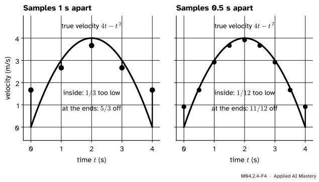
Often there is no formula at all, only measurements. Suppose the cart is timed once a second: its positions are 0, \({5/3}\), \({16/3}\), 9 and \({32/3}\) metres. At an inside time the central difference uses the samples either side. At \({t = 1}\) it gives \({(16/3 - 0)/2 = 8/3 \approx 2.67}\) m/s, at \({t = 2}\)\({(9 - 5/3)/2 = 11/3}\), and at \({t = 3}\) again \({8/3}\). The true velocities are 3, 4 and 3, so each estimate is \({1/3}\) too low. That is the \({h^2}\) error once more: the \({t^3/3}\) part of \({s(t)}\) makes the central difference \({h^2/3}\) too low with \({h = 1}\), and the \({2t^2}\) part is differenced exactly (exercise 2). At the two ends there is only one neighbour, so a one-sided difference has to do: at \({t = 0}\) it gives \({(5/3 - 0)/1 = 5/3}\), against the true 0.
M04.2.4-F4
numpy.gradient on the cart’s positions. Inside, central differences miss by \({h^2/3}\); at the ends, one-sided differences miss by much more. Halving the spacing cuts the inside error by four.
Code
First from scratch: the two differences, then the worked example, then a sweep over many steps.
def forward(f, x, h):return (f(x + h) - f(x)) / hdef central(f, x, h):return (f(x + h) - f(x - h)) / (2* h)cube =lambda x: x * x * xprint(" h forward central")for h in [0.1, 0.05]:print(f" {h:<6}{forward(cube, 1.0, h):.4f}{central(cube, 1.0, h):.4f}")
 h      forward   central
 0.1    3.3100    3.0100
 0.05   3.1525    3.0025
Now a step of \({10^{-1}}\), \({10^{-2}}\), and so on down to \({10^{-15}}\). The steps are written as decimal literals, which every computer reads the same way.
print(" h forward central")errors = {}for k inrange(1, 16): h =float(f"1e-{k}") errors[k] = (abs(forward(cube, 1.0, h) -3), abs(central(cube, 1.0, h) -3))print(f" 1e-{k:<4}{errors[k][0]:.1e}{errors[k][1]:.1e}")
The errors fall as the algebra says, ten times per step for the forward difference and a hundred times for the central one, then turn and grow. Your last digits may differ from these: they are rounding, which is the point.
Next, data. numpy.gradient takes samples and their positions and returns slope estimates: central differences inside, one-sided ones at the ends.
import numpy as npt = np.arange(5.0) # timed once a seconds =2* t**2- t**3/3# the cart's positions in metresprint("estimated, then true velocities:")print(np.round(np.gradient(s, t), 4))print(4* t - t**2)t_fine = np.linspace(0, 4, 41) # timed every 0.1 ss_fine =2* t_fine**2- t_fine**3/3inside_error = (np.gradient(s_fine, t_fine) - (4* t_fine - t_fine**2))[1:-1]print("inside error, samples 0.1 s apart:")print(np.round(inside_error.min(), 6), "to", np.round(inside_error.max(), 6))
estimated, then true velocities:
[1.6667 2.6667 3.6667 2.6667 1.6667]
[0. 3. 4. 3. 0.]
inside error, samples 0.1 s apart:
-0.003333 to -0.003333
When there is a formula, SciPy can estimate the derivative far more accurately. Its scipy.differentiate.derivative uses higher-order differences and shrinks the step until two estimates agree.
from scipy.differentiate import derivativeresult = derivative(lambda t: 2* t**2- t**3/3, 1.0)print(f"velocity at 1 s: {result.df:.12f}")print(f"its error estimate: {result.error:.0e}")
velocity at 1 s: 3.000000000000
its error estimate: 1e-14
Last, the gradient check: compare a derivative found by hand with a central difference, using the relative error \({\abs{a - n}/\max(\abs{a}, \abs{n})}\), where \(a\) is the hand formula and \(n\) the numerical estimate. Below, the running loss is checked against its correct slope and against a version that forgot the 2 in \({\tfrac{d}{dw} w^2}\).
def L(w):return7.5* w**2-23.5* w +18.5# the running lossdef slope_by_hand(w):return15* w -23.5def slope_with_a_bug(w):return7.5* w -23.5# forgot the factor 2def relative_error(f, dfdx, x, h=1e-5): numeric, analytic = central(f, x, h), dfdx(x)returnabs(analytic - numeric) /max(abs(analytic), abs(numeric))print(" w correct buggy")for w in [0.0, 1.0, 2.0]:print(f" {w:<5}{relative_error(L, slope_by_hand, w):.0e}{relative_error(L, slope_with_a_bug, w):.0e}")
The correct slope agrees to about \({10^{-11}}\) or better, the level of rounding: the central difference is exact on a quadratic (exercise 2). The buggy slope is off by 47 per cent at \({w = 1}\), a clear failure, yet it passes at \({w = 0}\), where both formulas happen to give \({-23.5}\). Check at several random points, never one.
Explore
This module’s interactive, the secant slider, lives in lesson M04.2.1. Its secant from \(P\) to \(Q\) is a forward difference for \({h > 0}\) and a backward one for \({h < 0}\). Press Central secant to add the secant from \({a - h}\) to \({a + h}\). With \({x^2}\) its slope is exactly 2 for every \(h\); with the cart it is \({3 - h^2/3}\); with \({\abs{x}}\) at 0 it is 0, a slope the corner does not have.
Pitfalls
M04.2.4-F5
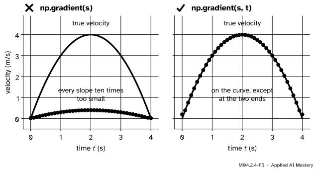
Wrong beside right. With samples 0.1 s apart, np.gradient(s) assumes a spacing of 1 and returns slopes ten times too small; np.gradient(s, t) uses the real times.
“A smaller step is always more accurate.”
Only until rounding takes over. For \({x^3}\) at 1 the forward difference with \({h = 10^{-12}}\) is off by about \({3 \times 10^{-4}}\), about as much as with \({h = 10^{-4}}\) and thousands of times more than with \({h = 10^{-8}}\). For a central difference a step near \({10^{-5}}\) or \({10^{-6}}\) is a good default, made larger in proportion when \(x\) itself is large.
“np.gradient(y) gives the derivative of \(y\).”
Only if the samples are 1 apart. Without the second argument NumPy assumes unit spacing, so with samples 0.1 s apart every slope comes out ten times too small: 0.2997 instead of 2.9967 at \({t = 1}\). Pass the sample positions, np.gradient(y, x), or the spacing.
“One gradient check that passes proves the slope right.”
A check at one point can pass by luck. The buggy slope \({7.5w - 23.5}\) agrees with the correct one at \({w = 0}\) and nowhere else. Check at several random points, and read the relative error, not the raw difference: below about \({10^{-7}}\) is reassuring, above \({10^{-2}}\) probably a bug.
“A gradient check works at every point.”
Not at a kink. At the corner of ReLU, the central difference straddles both sides and returns \({(h - 0)/(2h) = 1/2}\) for every \(h\), a slope that exists on neither side. Correct code that returns 0 or 1 there would fail the check, and for \({\abs{x}}\) the check returns 0, which would pass a slope that does not exist. Check away from kinks.
Check yourself
Recall
1. Write the forward and the central difference of \(f\) at \(x\) with step \(h\).
2. What are their exact errors for \({f(x) = x^3}\)?
Show answer
\({3xh + h^2}\) for the forward difference and \({h^2}\) for the central one.
3. What does halving \(h\) do to each error?
Show answer
It roughly halves the forward error and quarters the central error.
4. Why does the error grow again when \(h\) is very small?
Show answer
Each value of \(f\) is stored with about 16 significant digits. Subtracting two nearly equal values keeps their rounding errors, and dividing by a tiny \(h\) magnifies them to about \({10^{-16}/h}\).
5. What does a gradient check compare, and how?
Show answer
A derivative found by hand against a central difference, at several points, by their relative error \({\abs{a - n}/\max(\abs{a}, \abs{n})}\).
Exercises
1.★ By hand, estimate the slope of \({x^2}\) at \({x = 3}\) with \({h = 0.1}\), by the forward and the central difference. Compare with the true slope 6.
Show solution
\({3.1^2 = 9.61}\) and \({2.9^2 = 8.41}\). Forward: \({(9.61 - 9)/0.1 = 6.1}\), an error of \({0.1 = h}\). Central: \({(9.61 - 8.41)/0.2} = {1.2/0.2} = {6}\), exactly right.
2.★★ Show that the central difference is exact for every quadratic \({px^2 + qx + r}\), whatever the step, while the forward difference is off by \({ph}\). Use this to explain why numpy.gradient was off by exactly \({h^2/3}\) inside the cart’s samples.
Show solution
The constant \(r\) cancels, and \({(x+h)^2 - (x-h)^2 = 4xh}\), so the central difference is
\[
\frac{p\,(4xh) + q\,(2h)}{2h} = 2px + q ,
\]
the exact slope of the quadratic. The forward difference is \({2px + q + ph}\) (lesson 1, exercise 3). For the cart, \({s(t) = 2t^2 - t^3/3}\): the quadratic part is differenced exactly, and the cubic part \({-t^3/3}\) gives \({-\tfrac{1}{3}(3t^2 + h^2)}\), which is \({h^2/3}\) below its true slope \({-t^2}\). So the inside estimates are \({h^2/3}\) too low at every sample.
3.★★★ Compute the central difference at 0 of ReLU and of \({\abs{x}}\), for any \({h > 0}\). Explain why a gradient check exactly at a kink can mislead in both directions.
Show solution
ReLU: \({(\max(0, h) - \max(0, -h))/(2h)} = {(h - 0)/(2h)} = {1/2}\). Absolute value: \({(\abs{h} - \abs{-h})/(2h) = 0}\). Neither is a slope of the function at 0, which has none. If training code returns a one-sided slope of ReLU at 0, 1 or 0, its relative error against \({1/2}\) is 0.5 or 1, so correct code fails the check. For \({\abs{x}}\), code that wrongly claimed a slope of 0 at the corner would pass. Near a kink, test at points a few steps away from it.
Summary card
A computer estimates a slope from a short secant; look both ways and mind the rounding.
M04.2.4-F1
Forward against central.
Forward.\({(f(x+h) - f(x))/h}\), error proportional to \(h\): \({3xh + h^2}\) for \({x^3}\).
Central.\({(f(x+h) - f(x-h))/(2h)}\), error proportional to \({h^2}\): exactly \({h^2}\) for \({x^3}\).
Rounding. Below about \({10^{-8}}\) (forward) or \({10^{-6}}\) (central), smaller steps make things worse.
Libraries.np.gradient(y, x) for samples; scipy.differentiate.derivative(f, x).df for a function.
Gradient check. Relative error between the hand slope and a central difference, at several random points away from kinks.
Sources and next steps
Sources. Each was opened and checked against this lesson on 12 November 2026.
NumPy 2.5 reference, numpy.gradient: “second order accurate central differences in the interior points and either first or second order accurate one-sides (forward or backwards) differences at the boundaries”, unit spacing by default, and edge_order of 1 (the default) or 2.
SciPy 1.18 reference, scipy.differentiate.derivative: its defaults (order=8, initial_step=0.5, step_factor=2.0, maxiter=10) and the result’s df, error and success.
CS231n, Neural Networks Part 3: Learning and Evaluation, section Gradient Checks: use the centred formula, whose error is of order \({h^2}\) against \({h}\) for the forward one; a step of about \({10^{-5}}\); compare by relative error (above \({10^{-2}}\) probably wrong, below \({10^{-7}}\) good); beware precision problems with smaller steps, and kinks.
Marc Peter Deisenroth, A. Aldo Faisal and Cheng Soon Ong, Mathematics for Machine Learning, the remark “Verifying the Correctness of a Gradient Implementation” at the end of Section 5.2.2: compare a finite-difference approximation with the analytic gradient, with a small step such as \({10^{-4}}\).
Next. Module M04.3 Differentiation rules and the chain rule replaces limits by rules for powers, products and compositions, and checks each rule with the central difference built here.