\( \newcommand{\vect}[1]{\mathbf{#1}} \newcommand{\mat}[1]{\mathbf{#1}} \newcommand{\R}{\mathbb{R}} \newcommand{\E}{\mathbb{E}} \newcommand{\Prob}{\mathbb{P}} \newcommand{\T}{^{\top}} \newcommand{\norm}[1]{\lVert #1 \rVert} \newcommand{\abs}[1]{\lvert #1 \rvert} \newcommand{\ihat}{\mkern1mu\hat{\boldsymbol{\imath}}\mkern2mu} \newcommand{\jhat}{\mkern1mu\hat{\boldsymbol{\jmath}}\mkern2mu} \newcommand{\pd}[2]{\frac{\partial #1}{\partial #2}} \newcommand{\argmax}{\operatorname*{arg\,max}} \newcommand{\argmin}{\operatorname*{arg\,min}} \newcommand{\cdata}[1]{\class{c-data}{#1}} \newcommand{\cmodel}[1]{\class{c-model}{#1}} \newcommand{\ctruth}[1]{\class{c-truth}{#1}} \newcommand{\cgrad}[1]{\class{c-grad}{#1}} \newcommand{\closs}[1]{\class{c-loss}{#1}} \newcommand{\cparam}[1]{\class{c-param}{#1}} \newcommand{\csecond}[1]{\class{c-second}{#1}} \renewcommand{\,}{\mkern3mu} \)

From average rate to instantaneous rate

A speedometer shows a speed at one instant, yet speed is distance over time, which needs two instants. See how the slope of a secant line becomes the derivative as its second point slides in, and compute it for x squared and for a moving cart.

M04.2.1L1 Core25 minIn review

Before this lesson

M04.1 Limits and continuity M01.3 Functions and graphs

After this lesson you can

• Compute the average rate of change of a function over an interval, with its units, and read it as the slope of a secant line.
• Simplify the difference quotient of a polynomial and find its limit as the step h tends to 0.
• State the definition of the derivative at a point and interpret it as the slope of the tangent and as an instantaneous rate.
• Code the difference quotient in plain Python and NumPy and watch it settle as h shrinks.

In review. The maths and code on this page are checked by automated tests on every change, but an independent reader has not signed it off yet. Spot a mistake or a confusing step? Tell us.

The question

A car’s speedometer reads 50 kilometres per hour at this very instant. But speed is distance divided by time, and in a single instant the car covers no distance in no time: 0 divided by 0. So what number is the speedometer showing? Ask the same question of a loss instead of a car and you have the question a model trained by gradient descent asks at every step: how fast does the loss change as one weight moves?

Intuition

The average rate of change of a function over an interval is the change in its output divided by the change in its input: rise over run, as for a straight line in M01.3.2. On a graph it is the slope of a secant line, the straight line through the two points of the graph at the ends of the interval.

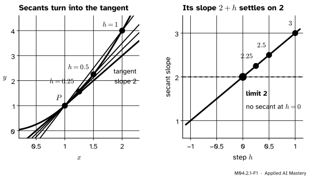
Take the running curve of this course, \({f(x) = x^2}\), and fix the point \({P = (1, 1)}\) on it. Put a second point \(Q\) on the curve a step \(h\) to the right, at \({x = 1 + h}\). With \({h = 1}\) the second point is \({(2, 4)}\), and the secant rises 3 over a run of 1: slope 3. Now slide \(Q\) in towards \(P\).

M04.2.1-F1

The secant from \({P = (1, 1)}\) to a second point \({h}\) further along. As \(h\) shrinks from 1 to 0.25 the secant pivots about \(P\) towards the green tangent line, and its slope \({2 + h}\) falls from 3 to 2.25 towards 2. At \({h = 0}\) itself there is no secant: the hollow circle.

With \({h = 0.5}\) the slope is 2.5, and with \({h = 0.25}\) it is 2.25. The secants pivot about \(P\) and settle on one line, the tangent line to the curve at \(P\). Its slope is the number the secant slopes close in on, 2. That number is the derivative of \({x^2}\) at \({x = 1}\): the rate of change at one point, not over an interval.

Two things in the picture matter. The step never reaches 0: with \(Q\) on top of \(P\) there is one point, and one point fixes no line. And yet the slopes come as close to 2 as we like. A value that is approached but never used is exactly what a limit describes (M04.1), and the hole in the right panel is the hole that M04.1.1 met in its first table.

Build it up

The same idea, slowly, on a quantity with units. The running trip of this course is a cart that starts and stops within four seconds (an invented example). After \(t\) seconds it is \({s(t)}\) metres from its start, where \({s(t) = 2t^2 - t^3/3}\).

Step 1. An average rate from a table. The cart’s position each second, and the average velocity over the second that follows:

\(t\) (s)	\({s(t)}\) (m)	average over the next second (m/s)
0	0	\({5/3 \approx 1.67}\)
1	\({5/3}\)	\({11/3 \approx 3.67}\)
2	\({16/3}\)	\({11/3 \approx 3.67}\)
3	\(9\)	\({5/3 \approx 1.67}\)
4	\({32/3}\)

Each average is a change in position divided by a change in time, so it is measured in metres per second. That is the rule for every rate: its units are units of output per unit of input. Over the whole trip the cart covers \({32/3}\) metres in 4 seconds, an average of \({8/3 \approx 2.67}\) m/s.

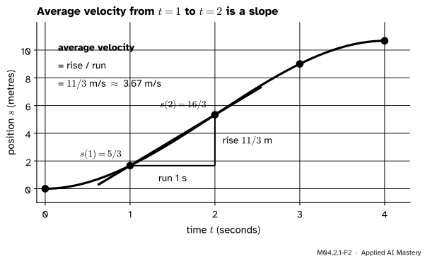
Step 2. The average is a slope. Plot position against time. The average velocity from \({t = 1}\) to \({t = 2}\) is the rise of the graph, \({16/3 - 5/3 = 11/3}\) metres, over the run of 1 second: the slope of the secant through the two points.

M04.2.1-F2

The average velocity over one second is the slope of the secant: a rise in metres over a run in seconds, so its units are metres per second.

Step 3. Shrink the run. Keep the start at \({t = 1}\) and end at \({t = 1 + h}\). The average velocity over that interval is

\[ \frac{s(1+h) - s(1)}{h} . \]

With \({h = 0.5}\): \({s(1.5) = 4.5 - 1.125 = 3.375}\), so the average is \({(3.375 - 5/3)/0.5 \approx 3.4167}\) m/s. With \({h = 0.1}\) it is about 3.0967, and with \({h = 0.01}\) about 3.00997. The averages settle near 3.

Step 4. The instant is a limit. The cart’s velocity at the instant \({t = 1}\), what its speedometer shows, is the number these averages close in on as \(h\) shrinks to 0. The step may be as small as we like, but never 0, where the quotient would be \({0/0}\).

The formal statement

NoteDefinition: difference quotient and derivative

Let \(f\) be a function, \(a\) a point of its domain, and \({h \neq 0}\) a step with \({a + h}\) in the domain too. The difference quotient

\[ \cmodel{\frac{f(a+h) - f(a)}{\cparam{h}}} \]

is the average rate of change of \(f\) from \(a\) to \({a + h}\): the slope of the secant through \({(a, f(a))}\) and \({(a + h, f(a + h))}\). The derivative of \(f\) at \(a\) is its limit,

\[ \cgrad{f'(a)} = \lim_{h \to 0} \frac{f(a+h) - f(a)}{h} , \]

provided the limit exists. Then \(f\) is differentiable at \(a\), and the tangent line to the graph at \({(a, f(a))}\) is the line through that point with slope \({f'(a)}\).

Read \({f'(a)}\) as “f prime of a”. It is the instantaneous rate of change of \(f\) at \(a\). When \(f\) is a position and the input is time, it is the velocity: \({v(a) = s'(a)}\). Its units are those of the quotient, units of output per unit of input. For a loss \(L\) and a weight \(w\), \({L'(w)}\) is measured in loss per unit of weight.

The derivative of \({x^2}\) at 1, every step shown. Multiply out the square, subtract \({f(1) = 1}\), then divide by \(h\), which is allowed because \({h \neq 0}\):

\[ \begin{aligned} f(1+h) &= (1+h)^2 \\ &= 1 + 2h + h^2 , \\ f(1+h) - f(1) &= 2h + h^2 , \\ \frac{f(1+h) - f(1)}{h} &= 2 + h . \end{aligned} \]

For every \({h \neq 0}\) the quotient equals \({2 + h}\). As \(h\) tends to 0, \({2 + h}\) tends to 2, because a polynomial in \(h\) tends to its value at \({h = 0}\) (M04.1.2). So \({f'(1) = 2}\), the slope of the tangent in the anchor picture.

The cancelled \(h\) is the whole trick. Before cancelling, the quotient is \({0/0}\) at \({h = 0}\) and has no value there. After cancelling it is a plain polynomial whose limit we can read off. This is the first limit of M04.1 in disguise: write \({x = 1 + h}\) and the secant slope becomes \({(x^2 - 1)/(x - 1)}\), the function with a hole at height 2 that M04.1.1 tabulated.

Go deeper: the same limit written with x instead of h

Put \({x = a + h}\). Then \({h = x - a}\), and \(h\) tends to 0 exactly when \(x\) tends to \(a\), so

\[ f'(a) = \lim_{x \to a} \frac{f(x) - f(a)}{x - a} . \]

The two forms are one definition: the first measures the step, the second names the second point. For \({x^2}\) at 1 the second form gives \({(x^2 - 1)/(x - 1) = x + 1}\) for \({x \neq 1}\), which tends to 2. OpenStax writes the derivative both ways (its equations 3.5 and 3.6).

Worked example

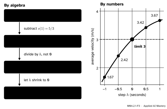
What does the cart’s speedometer read at \({t = 1}\)? First the starting position: \({s(1) = 2 - 1/3 = 5/3}\) metres. Then expand \({s(1 + h)}\), using \({(1+h)^2 = 1 + 2h + h^2}\) and \({(1+h)^3 = 1 + 3h + 3h^2 + h^3}\):

\[ \begin{aligned} s(1+h) &= 2(1+h)^2 - \tfrac{1}{3}(1+h)^3 \\ &= (2 + 4h + 2h^2) \\ &\quad - \tfrac{1}{3}(1 + 3h + 3h^2 + h^3) \\ &= \tfrac{5}{3} + 3h + h^2 - \tfrac{1}{3}h^3 . \end{aligned} \]

The last line collects like terms: \({2 - 1/3 = 5/3}\), \({4h - h = 3h}\) and \({2h^2 - h^2 = h^2}\). Subtract \({s(1) = 5/3}\) to get the rise, then divide by the run \(h\):

\[ \begin{aligned} s(1+h) - s(1) &= 3h + h^2 - \tfrac{1}{3}h^3 \\ \frac{s(1+h) - s(1)}{h} &= 3 + h - \tfrac{1}{3}h^2 . \end{aligned} \]

As \(h\) tends to 0, \({h}\) and \({h^2/3}\) both tend to 0, so the average velocity tends to 3 metres per second: the cart’s speedometer reads 3 m/s at \({t = 1}\). At the whole seconds 0 to 4 it reads 0, 3, 4, 3 and 0 m/s; exercise 2 finds the 4, and lesson 4 the formula \({4t - t^2}\) behind all of them.

M04.2.1-F3

The worked example as a trace. The algebra (left) turns the average velocity into \({3 + h - h^2/3}\); the numbers (right) close in on 3 from below for negative steps and from above for positive ones.

Check the formula against a number found directly. For \({h = 0.5}\) it gives \({3 + 0.5 - 0.25/3 \approx 3.4167}\), the value of Step 3. For \({h = -0.5}\) it gives \({3 - 0.5 - 0.25/3 \approx 2.4167}\), the average over the half second before \({t = 1}\). The averages over short steps after \({t = 1}\) are above 3 and those before it below 3, because the cart is speeding up: it covers more ground in the moment after \({t = 1}\) than in the moment before.

Code

First from scratch. The difference quotient is one line, and it works for any function.

def difference_quotient(f, a, h):
    """Average rate of change of f from a to a + h: the slope of a secant."""
    return (f(a + h) - f(a)) / h

def f(x):
    return x * x                      # the running curve

def s(t):
    return 2 * t**2 - t**3 / 3        # the running trip: position in metres

print(" h       x^2 at 1   cart (m/s)")
for h in [1, 0.5, 0.1, 0.01, 0.001]:
    print(f" {h:<7} {difference_quotient(f, 1, h):<10.6f} {difference_quotient(s, 1, h):.6f}")

 h       x^2 at 1   cart (m/s)
 1       3.000000   3.666667
 0.5     2.500000   3.416667
 0.1     2.100000   3.096667
 0.01    2.010000   3.009967
 0.001   2.001000   3.001000

The columns match \({2 + h}\) and \({3 + h - h^2/3}\). Printed with all their digits, some floats show a stray last digit: try difference_quotient(f, 1, 0.1), which prints something like 2.100000000000002. That is rounding in the computer’s arithmetic, the subject of lesson 4, not a fault in the algebra. Python’s exact fractions confirm it:

from fractions import Fraction

exact = difference_quotient(f, Fraction(1), Fraction(1, 10))
print("slope from 1 to 1.1, exactly:", exact)

slope from 1 to 1.1, exactly: 21/10

NumPy does the same computation for many steps at once, on both sides of the point. The functions above work unchanged on arrays.

import numpy as np

hs = np.array([0.5, 0.1, 0.01, -0.01, -0.1, -0.5])
slopes = (f(1 + hs) - f(1)) / hs
velocities = (s(1 + hs) - s(1)) / hs
print("  h      slope    velocity (m/s)")
for h, m, v in zip(hs, slopes, velocities):
    print(f"{h:6.2f}   {m:.4f}   {v:.4f}")

  h      slope    velocity (m/s)
  0.50   2.5000   3.4167
  0.10   2.1000   3.0967
  0.01   2.0100   3.0100
 -0.01   1.9900   2.9900
 -0.10   1.9000   2.8967
 -0.50   1.5000   2.4167

A table like this is evidence, not proof: it shows the quotient near 2, but only the algebra shows that it is exactly \({2 + h}\) and so has limit exactly 2.

Explore

M04.2-X1

Secant slider

Drag the orange point \(Q\) along the curve towards \(P\), or slide the step \(h\). The vermillion secant turns towards the green tangent while the read-out prints its slope beside the limit. Halve h steps the second point in; Play slides it in smoothly.

Things to try:

1. With \({x^2}\) at 1, set \({h = 0.5}\) and press Halve h four times. How far is each slope from 2?
2. Press Flip side to put \(Q\) on the left. Which side gives slopes above 2?
3. Choose the cart. In what units is the slope, and what does it approach?
4. Choose \({\abs{x}}\) at 0 and flip sides. Lesson M04.2.3 explains what you see.

Pitfalls

M04.2.1-F4

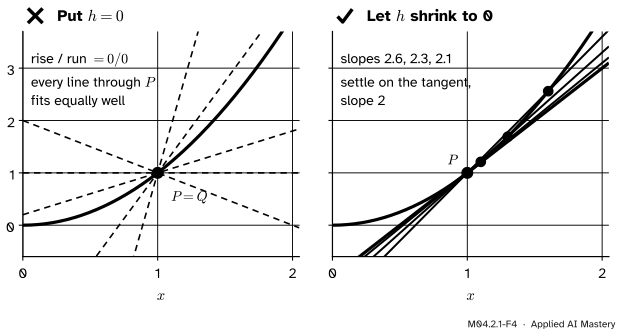
Wrong beside right. Setting \({h = 0}\) leaves one point, and one point fixes no line. Letting \(h\) shrink gives secants that settle on one line, the tangent.

“To get the derivative, just put \({h = 0}\) in the quotient.”

That gives \({(f(a) - f(a))/0 = 0/0}\), which has no value: the two points are the same point, and every line through it is equally good. Simplify first, cancelling the \(h\) (for \({x^2}\) at 1, \({(2h + h^2)/h = 2 + h}\)), and only then let \(h\) tend to 0.

“The derivative is the slope over a tiny interval, such as \({h = 0.001}\).”

Any fixed \(h\) gives an average over an interval. For \({x^2}\) at 1 the quotient with \({h = 0.001}\) is 2.001, not 2. The derivative is the limit, the one number every small step closes in on. A computer works with a small \(h\) and accepts a small error, which lesson 4 measures.

“The average velocity is the average of the starting and finishing speeds.”

The cart starts and ends at rest, so that recipe gives \({(0 + 0)/2 = 0}\) m/s for the whole trip. Yet it covered \({32/3}\) metres in 4 seconds, an average of \({8/3 \approx 2.67}\) m/s. An average rate is total change over total time: the slope of the secant, not a mean of two slopes.

“A rate has the units of the thing that changes.”

A rate is a quotient, so it carries a “per”. The cart’s velocity is in metres per second, not metres. In machine learning the slope of a loss with respect to a weight is in loss per unit of weight, so its size depends on the units in which the weight is measured, just as a speed in metres per second differs from the same speed in kilometres per hour.

Check yourself

Recall

1. What does the difference quotient \({(f(a+h) - f(a))/h}\) measure, on a graph and as a rate?

Show answer

The slope of the secant through \({(a, f(a))}\) and \({(a+h, f(a+h))}\), which is the average rate of change of \(f\) from \(a\) to \({a + h}\).

2. Write the definition of the derivative of \(f\) at \(a\).

Show answer

\({f'(a)} = {\lim_{h \to 0} (f(a+h) - f(a))/h}\), provided the limit exists.

3. For \({f(x) = x^2}\), what is the secant slope from 1 to \({1 + h}\), and what is \({f'(1)}\)?

Show answer

The slope is \({2 + h}\) for every \({h \neq 0}\), and \({f'(1) = 2}\).

4. Why can you not simply put \({h = 0}\) in the difference quotient?

Show answer

It becomes \({0/0}\), which has no value: the two points coincide, and one point fixes no line. The derivative is the limit as \(h\) tends to 0, found after cancelling \(h\).

5. A position is in metres and time in seconds. What are the units of the average velocity and of the instantaneous velocity?

Show answer

Metres per second for both: a rate has units of output per unit of input.

Exercises

1. ★ For \({f(x) = x^2}\), find the average rate of change from \({x = 2}\) to \({x = 3}\), and from \({x = 2}\) to \({x = 2.1}\). What do you expect \({f'(2)}\) to be?

Show solution

From 2 to 3: \({(9 - 4)/(3 - 2) = 5}\). From 2 to 2.1: \({(4.41 - 4)/0.1 = 4.1}\). In general \({((2+h)^2 - 4)/h} = {(4h + h^2)/h} = {4 + h}\), so the averages are \({4 + h}\) and \({f'(2) = 4}\).

2. ★★ From the definition, find the cart’s velocity at \({t = 2}\).

Show solution

First \({s(2) = 8 - 8/3 = 16/3}\). Using \({(2+h)^2 = 4 + 4h + h^2}\) and \({(2+h)^3 = 8 + 12h + 6h^2 + h^3}\), the two parts of \({s(2+h)}\) are

\[ \begin{aligned} 2(2+h)^2 &= 8 + 8h + 2h^2 , \\ \tfrac{1}{3}(2+h)^3 &= \tfrac{8}{3} + 4h \\ &\quad + 2h^2 + \tfrac{1}{3}h^3 . \end{aligned} \]

Subtract the second from the first: \({s(2+h) = 16/3 + 4h - h^3/3}\). The \({h^2}\) terms cancel (\({2h^2 - 2h^2}\)). So the rise is \({4h - h^3/3}\), the average velocity is \({4 - h^2/3}\), and its limit is 4 m/s, the top speed of the trip. Here the averages fall short of 4 on both sides, since \({h^2/3}\) is never negative.

3. ★★★ Show that for any quadratic \({f(x) = px^2 + qx + r}\) the secant slope from \(a\) to \({a + h}\) is \({2pa + q + ph}\). Deduce \({f'(a)}\), and the exact gap between the secant slope and the derivative.

Show solution

Expand: \({f(a+h)} = {p\,(a^2 + 2ah + h^2)} + {q\,(a + h)} + {r}\). Subtracting \({f(a) = pa^2 + qa + r}\) leaves

\[ \begin{aligned} &f(a+h) - f(a) \\ &\quad= 2pah + ph^2 + qh , \\ &\frac{f(a+h) - f(a)}{h} \\ &\quad= 2pa + q + ph . \end{aligned} \]

As \(h\) tends to 0 this tends to \({2pa + q}\), so \({f'(a) = 2pa + q}\), and the secant slope exceeds the derivative by exactly \({ph}\). For \({x^2}\) (\({p = 1}\), \({q = 0}\)) this is \({2a + h}\), which is \({2 + h}\) at \({a = 1}\). For the running loss \({L(w) = 7.5w^2 - 23.5w + 18.5}\) it gives \({L'(w) = 15w - 23.5}\), the slope the next lesson uses.

Summary card

The derivative is the limit of secant slopes: the rate at one instant.

M04.2.1-F1

Secants turn into the tangent.

• Average rate. \({(f(a+h) - f(a))/h}\), the slope of a secant, in units of output per unit of input.
• Derivative. \({f'(a)}\) is the limit of \({(f(a+h) - f(a))/h}\) as \({h \to 0}\): cancel \(h\) first, then let it shrink.
• Running curve. For \({x^2}\) at 1 the secant slope is \({2 + h}\), so \({f'(1) = 2}\).
• Running trip. The cart’s average velocity over \({[1, 1 + h]}\) is \({3 + h - h^2/3}\), so its velocity at \({t = 1}\) is 3 m/s.

Sources and next steps

Sources. Each was opened and checked against this lesson on 12 November 2026.

• Gilbert Strang and Edwin Herman, Calculus Volume 1, Section 3.1 Defining the Derivative, OpenStax. The difference quotient (equations 3.1 and 3.2), the tangent slope as its limit (3.4), the derivative in both forms (3.5 and 3.6), and average and instantaneous velocity (3.7 and 3.8).
• Matthew Boelkins, Active Calculus, Section 1.1 How do we measure velocity?, where the average velocity on an interval is the slope of the line through two points of the position graph and the instantaneous velocity is what averages over shrinking intervals approach, before limits are defined; and Section 1.5, on the units of a derivative, “units of output per unit of input”.
• Marc Peter Deisenroth, A. Aldo Faisal and Cheng Soon Ong, Mathematics for Machine Learning, Section 5.1: the difference quotient as the slope of a secant (Definition 5.1) and the derivative as its limit, where the secant becomes a tangent (Definition 5.2).
• David Jerison, MIT OpenCourseWare 18.01SC, Unit 1, Session 1: Introduction to Derivatives, the derivative as the slope of a tangent line and the limit of secants, and Session 3, the derivative as a rate of change.

Next. M04.2.2 The tangent line and linear approximation uses the tangent to estimate values near a point, and reads the derivative of a loss as a sensitivity.

This lesson unlocks

M04.2.2 The tangent line and linear approximation

Your progress is saved in this browser only. No account, no tracking.