Put the two partial derivatives side by side and they make an arrow on the map: the gradient. It points the way a function climbs fastest, its length is that fastest slope, and at right angles to it, along the contour line, the function stays level.
Form the gradient of a function of two variables and draw it as an arrow on the contour map.
Use the linear approximation in each input to estimate how much f changes for a small step in any direction.
Derive that the slope in the direction at angle θ is largest along the gradient, equal to its length, and zero along the contour line.
Explain why a step against the gradient lowers a loss fastest, and why it need not point at the lowest point.
Check a gradient with central differences, a scan over directions and scipy.optimize.approx_fprime.
In review. The maths and code on this page are checked by automated tests on every change, but an independent reader has not signed it off yet. Spot a mistake or a confusing step? Tell us.
The question
On a hillside in fog you can feel the slope under your feet in two directions, east and north: those are the two partial derivatives. But which way is straight uphill, and how steep is it? Training faces the same question at every step. Of all the small changes it could make to two parameters at once, which lowers the loss the most?
From the last lesson
1. What are \({\pd{f}{x}}\) and \({\pd{f}{y}}\) for \({f(x, y) = x^2 + 2y^2}\) at \({(1, 1)}\)?
2. What is the partial derivative of the squared error \({(wx + b - y)^2}\) with respect to \(b\)?
Show answer
\({2(wx + b - y)}\): twice the residual.
Intuition
Write the two partial derivatives at a point side by side and you get a pair of numbers, the same shape as the point itself. Draw the pair as an arrow on the map, starting at the point: this arrow is the gradient, written \({\nabla f}\) (“nabla \(f\)”). At \({(1, 1)}\) on the running bowl it is \({(2, 4)}\).
M04.10.3-F1
The gradient at several points of the running bowl, each arrow drawn at a quarter of its length. Every arrow points straight uphill, across the contour lines; along the contour line through \({(1, 1)}\) the ground is level.
The picture makes three claims, and this lesson proves them. The gradient points the way the function climbs fastest. Its length is that fastest slope. And at right angles to it, along the contour line, the function does not change at all. Turn the arrow round and you have the way down, the direction in which gradient descent moves a model’s parameters.
Build it up
Step 1. A small step, in two moves. From \({(1, 1)}\) step to \({(1.1, 1.1)}\), and do it in two moves. First move \(x\) alone, from 1 to 1.1. Along the slice \({y = 1}\) the linear approximation of M04.2.2 says that \(f\) changes by about \({\pd{f}{x} \times \Delta x} = {2 \times 0.1} = {0.2}\). Then move \(y\) alone, from 1 to 1.1. The slope \({\pd{f}{y} = 4y}\) does not depend on \(x\), so it is still 4, and \(f\) changes by about \({4 \times 0.1 = 0.4}\). Altogether, about 0.6. The truth is \({f(1.1, 1.1)} = {1.21 + 2.42} = {3.63}\), a rise of 0.63. In general,
\[
\Delta f \approx \pd{f}{x}\,\Delta x + \pd{f}{y}\,\Delta y .
\]
For the bowl the change is exactly \({2\,\Delta x + 4\,\Delta y + \Delta x^2 + 2\,\Delta y^2}\), so the gap, here \({0.01 + 0.02 = 0.03}\), shrinks like the square of the step.
Step 2. A step in any direction. A step of length \(s\) at angle \(\theta\), measured anticlockwise from the \(x\) axis, moves \(x\) by \({s\cos\theta}\) and \(y\) by \({s\sin\theta}\) (M01.5). Write \(p\) and \(q\) for the two partial derivatives at the point. Then
\[
\Delta f \approx s\,(p\cos\theta + q\sin\theta) .
\]
Dividing by the length \(s\) gives the slope in that direction, \({p\cos\theta + q\sin\theta}\). East, \({\theta = 0}\), gives \(p\); north, \({\theta = 90^\circ}\), gives \(q\), as it must.
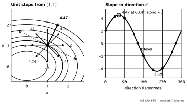
Step 3. Try every direction. At \({(1, 1)}\) the slope in direction \(\theta\) is \({2\cos\theta + 4\sin\theta}\): 2 to the east, 4 to the north, \({6/\sqrt{2} \approx 4.24}\) to the north-east, \(-2\) to the west, \(-4\) to the south.
M04.10.3-F2
The slope at \({(1, 1)}\) in each direction. It is a wave in \(\theta\): highest, 4.47, along the gradient at 63.4°, zero along the contour line, and lowest, \(-4.47\), straight against the gradient.
The largest value is a little above 4.24, somewhere between north-east and north. The next section finds it exactly.
The formal statement
NoteDefinitions: the gradient and the slope in a direction
The gradient of \(f\) at \((x, y)\) is the pair of its partial derivatives, in the order of the inputs:
A step of length \(s\) in the direction \(\theta\) ends at \({(x_s, y_s)} = {(x + s\cos\theta,\; y + s\sin\theta)}\). The slope of \(f\) in the direction \(\theta\) at \((x, y)\) is
For a function whose partial derivatives change smoothly, as every polynomial’s do, with \({p = \pd{f}{x}}\) and \({q = \pd{f}{y}}\) at the point,
\[
D_\theta f = p\cos\theta + q\sin\theta .
\]
If \({\nabla f \neq (0, 0)}\), write \({r = \sqrt{p^2 + q^2}}\) for its length. Then the largest slope is \(r\), along \({\nabla f}\); the smallest is \(-r\), straight against it; and the slope is 0 in the two directions at right angles to it. If \({\nabla f = (0, 0)}\), every direction has slope 0.
The formula for \({D_\theta f}\) is Step 2 made exact, in the limit of a short step (block below).
Proof of the rest. Any arrow is its length times the cosine and sine of its angle (M01.5), so write the gradient as \({p = r\cos\varphi}\) and \({q = r\sin\varphi}\), where \(\varphi\) is its angle. The angle \({-\varphi}\) turns clockwise (M01.5.2) and lands on the mirror image, in the \(x\) axis, of the point at angle \(\varphi\), so \({\cos(-\varphi) = \cos\varphi}\) and \({\sin(-\varphi) = -\sin\varphi}\). The cosine angle-addition formula of M01.5.4, used for the angles \(\theta\) and \({-\varphi}\), then gives \({\cos(\theta - \varphi)} = {\cos\theta\cos\varphi + \sin\theta\sin\varphi}\). So
A cosine is at most 1, and equals 1 only when \({\theta - \varphi}\) is 0 (or a whole turn), so the largest slope is \(r\), when \({\theta = \varphi}\): along the gradient. A cosine is at least \(-1\), reached when \({\theta = \varphi + 180^\circ}\): the smallest slope is \(-r\), straight against the gradient. And the cosine is zero when \({\theta = \varphi \pm 90^\circ}\): at right angles to the gradient, the slope is 0. The calculus of M04.4 agrees: \({D_\theta f}\) as a function of \(\theta\) has derivative \({-r\sin(\theta - \varphi)}\) (M04.3.2), zero at \({\theta = \varphi}\) and at \({\theta = \varphi + 180^\circ}\), and second derivative \({-r\cos(\theta - \varphi)}\), which is negative at the first, a maximum, and positive at the second, a minimum (M04.4.2).
The contour line. Walking along the contour line through a point, \(f\) does not change at all, so the slope in the contour line’s direction is 0. The only directions with slope 0 are the two at right angles to the gradient. So the gradient crosses the contour line at a right angle, and \({-\nabla f}\) is the direction of steepest descent.
Go deeper: why two slopes are enough, and when they are not
Name the three corners of the two-move path: the start \({P = (x, y)}\), the point \({Q = (x + \Delta x, y)}\) reached by moving \(x\) alone, and the end \({R = (x + \Delta x, y + \Delta y)}\). Then
The first bracket is a step along the slice through \(P\), about \({\pd{f}{x}(P)\,\Delta x}\). The second is a step in \(y\) alone, but taken from \(Q\), so it is about \({\pd{f}{y}(Q)\,\Delta y}\). When the partial derivatives change smoothly, \({\pd{f}{y}(Q)}\) is close to \({\pd{f}{y}(P)}\) and the two moves add up as in Step 1. The function \({xy/(x^2 + y^2)}\) of lesson 2 breaks this at the origin: both slopes are 0 there, yet along the diagonal the function jumps to \(\tfrac12\). Course M05 gives the general statement.
Worked example
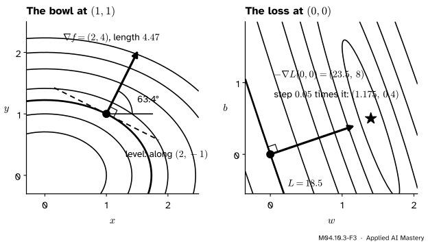
The bowl at \({(1, 1)}\). The gradient is \({(2, 4)}\), of length \({\sqrt{4 + 16} = \sqrt{20} \approx 4.47}\). Its angle has \({\tan\varphi = 4/2 = 2}\), so \({\varphi \approx 63.4^\circ}\). So the steepest climb from \({(1, 1)}\) is 4.47 per unit step, steeper than either axis direction. The level directions are at \({63.4^\circ \pm 90^\circ}\), along \({(2, -1)}\) and \({(-2, 1)}\): indeed \({2 \cdot 2 + 4 \cdot (-1) = 0}\). Check against the contour line \({x^2 + 2y^2 = 3}\) through the point: moving \(t\) along \({(2, -1)}\) gives
With \(b\) held constant, the six terms differentiate to \({15w}\), \({5b}\), 0, \({-23.5}\), 0 and 0; with \(w\) held constant, to 0, \({5w}\), \({2b}\), 0, \({-8}\) and 0:
At \({(0, 0)}\) the gradient is \({\nabla L = (-23.5, -8)}\). Both entries are negative: the loss falls as \(w\) grows and as \(b\) grows. The steepest way down is \({-\nabla L = (23.5, 8)}\): raise both, \(w\) about three times as fast as \(b\). Its slope is \({-\sqrt{23.5^2 + 8^2} = -\sqrt{616.25} \approx -24.8}\). This is the first step of gradient descent in ML01.5.2: with a learning rate of 0.05 it moves \({(0, 0)}\) to \({(1.175, 0.4)}\).
M04.10.3-F3
The worked example as a trace. On the bowl the gradient at \({(1, 1)}\) is 4.47 long and meets the contour line at a right angle. On the loss the way down from \({(0, 0)}\) is \({(23.5, 8)}\); a step of 0.05 times it lands near the star.
Code
First from scratch: the gradient by central differences, its length and its angle.
Now test the claim directly. Take a tiny step of length \({s = 10^{-6}}\) in each of the 360 whole degrees, measure the slope as rise over step, and see which direction wins.
def slope_towards(f, x, y, degrees, s=1e-6): a = math.radians(degrees)return (f(x + s * math.cos(a), y + s * math.sin(a)) - f(x, y)) / sslopes = [slope_towards(bowl, 1, 1, d) for d inrange(360)]steepest =max(range(360), key=lambda d: slopes[d])level =sorted(range(360), key=lambda d: abs(slopes[d]))[:2]print("steepest climb at", steepest, "degrees, slope", round(slopes[steepest], 4))print("steepest descent at", min(range(360), key=lambda d: slopes[d]), "degrees")print("closest to level at", sorted(level), "degrees")
steepest climb at 63 degrees, slope 4.472
steepest descent at 243 degrees
closest to level at [153, 333] degrees
The scan agrees with the formula: the best whole degree is 63, beside the exact 63.4°, and its slope is within 0.001 of \({\sqrt{20}}\). SciPy has a ready-made finite-difference gradient, scipy.optimize.approx_fprime. It takes the point as an array and uses forward differences with a tiny step, so its last digits wobble.
import numpy as npfrom scipy.optimize import approx_fprimex = np.array([1.0, 2.0, 3.0, 4.0])y = np.array([2.0, 3.0, 5.0, 6.0])loss =lambda v: np.mean((v[0] * x + v[1] - y) **2) # v = (w, b)print("bowl at (1, 1):", np.round(approx_fprime(np.array([1.0, 1.0]), lambda v: bowl(*v)), 4))print("loss at (0, 0):", np.round(approx_fprime(np.array([0.0, 0.0]), loss), 4))
bowl at (1, 1): [2. 4.]
loss at (0, 0): [-23.5  -8. ]
Explore
M04.10-X1
Slope compass
Drag the orange point over the contour map, or set it with the sliders. The side panels show the two slices through the point with their tangent lines, and the dial below them shows the slope in every direction. Turn the direction slider: the slope is largest along the green arrow and zero along the contour line. Then pick the loss or the saddle and press To the flat point.
Pitfalls
M04.10.3-F4
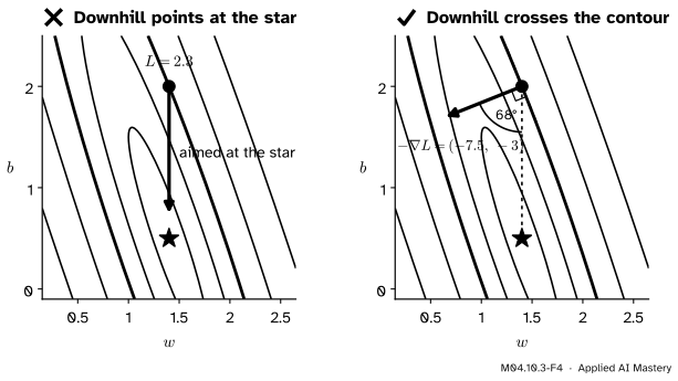
Wrong beside right, at \({(1.4, 2)}\) on the loss, straight above the lowest point. The steepest way down points mostly left, 68° away from the star.
“Minus the gradient points at the lowest point.”
It points straight downhill from where you stand, at a right angle to the contour line. At \({(1.4, 2)}\) the gradient is \({(7.5, 3)}\), so the way down is \({(-7.5, -3)}\), mostly towards smaller \(w\), while the lowest point is straight below. The two directions are 68° apart. In a long, narrow valley the steepest way down mostly crosses the valley rather than following it, which is why gradient descent zigzags there (ML01.5.3).
“The slope along the diagonal is the sum of the two partial derivatives.”
A unit step at 45° moves each input by only \({1/\sqrt{2} \approx 0.71}\), so at \({(1, 1)}\) the slope is \({(2 + 4)/\sqrt{2} \approx 4.24}\), not 6. No direction has a slope bigger than the length of the gradient, here 4.47.
“The gradient is an arrow on the surface.”
It is a pair of numbers with the shape of the input, drawn on the map of the inputs. Its length is a slope, height gained per unit of distance on the map. For a loss, \({\nabla L}\) has one entry per parameter.
Check yourself
Recall
1. What is the gradient of \({f(x, y)}\)?
Show answer
The pair of partial derivatives, \({\nabla f = \big(\pd{f}{x}, \pd{f}{y}\big)}\), drawn as an arrow on the map of the inputs.
2. About how much does \(f\) change for a small step \({(\Delta x, \Delta y)}\)?
Show answer
About \({\pd{f}{x}\,\Delta x + \pd{f}{y}\,\Delta y}\).
3. In which direction is the slope of \(f\) largest, and how large is it?
Show answer
Along the gradient, and the slope there is the gradient’s length, \({\sqrt{p^2 + q^2}}\).
4. Which directions have slope zero, and what are they on the map?
Show answer
The two at right angles to the gradient: the directions of the contour line through the point.
5. Why does gradient descent step along \({-\nabla L}\)?
Show answer
Because it is the direction of steepest descent. The slope there is minus the length of the gradient, the most negative of all directions, so a small step along it lowers the loss most.
Exercises
1.★ For the running bowl, find \({\nabla f(2, -1)}\), its length, and the slopes in the directions \({\theta = 0}\) and \({\theta = 90^\circ}\).
Show solution
\({\nabla f} = {(2x, 4y)} = {(4, -4)}\), of length \({\sqrt{16 + 16} = \sqrt{32} \approx 5.66}\). The slope to the east is \({\pd{f}{x} = 4}\) and to the north \({\pd{f}{y} = -4}\): northwards the bowl falls, because \({(2, -1)}\) is south of the centre.
2.★★ From \({(1, 1)}\) on the bowl, estimate \({f(1.02, 0.97)}\) with the linear approximation, and compare with the true value.
Show solution
\({\Delta x = 0.02}\) and \({\Delta y = -0.03}\), so \({\Delta f} \approx {2 \times 0.02 + 4 \times (-0.03)} = {0.04 - 0.12} = {-0.08}\), giving 2.92. The truth is \({1.02^2 + 2 \times 0.97^2} = {1.0404 + 1.8818} = {2.9222}\). The gap, 0.0022, is exactly \({\Delta x^2 + 2\,\Delta y^2} = {0.0004 + 0.0018}\).
3.★★★ On the loss at \({(w, b) = (1, 0)}\), find \({\nabla L}\), the direction and slope of steepest descent, and a direction in which \(L\) is level. Why does the first entry equal the slope of the running loss at \({w = 1}\)?
Show solution
\({\nabla L(1, 0)} = {(15 - 23.5,\; 5 - 8)} = {(-8.5, -3)}\). Steepest descent is along \({(8.5, 3)}\), raising both \(w\) and \(b\), with slope \({-\sqrt{72.25 + 9}} = {-\sqrt{81.25}} \approx {-9.01}\). A level direction is at right angles to the gradient, for example \({(3, -8.5)}\): \({-8.5 \times 3 + (-3) \times (-8.5) = 0}\).
\({\pd{L}{w}}\) at \({(1, 0)}\) is the slope of the slice \({b = 0}\), and that slice is the running loss \({7.5w^2 - 23.5w + 18.5}\), whose slope at \({w = 1}\) is \({15 - 23.5 = -8.5}\) (M04.2.2).
Summary card
The gradient is the arrow of steepest climb: its direction is straight uphill and its length is the slope there.
M04.10.3-F1
Uphill across, level along.
The gradient \({\nabla f}\) is the pair of partial derivatives, an arrow on the map.
For a small step, \({\Delta f} \approx {\pd{f}{x}\,\Delta x} + {\pd{f}{y}\,\Delta y}\).
Slope in direction \(\theta\): \({p\cos\theta + q\sin\theta}\), which is \({r\cos(\theta - \varphi)}\).
Largest along \({\nabla f}\), equal to its length; zero along the contour line.
Bowl at \({(1, 1)}\): \({(2, 4)}\), length 4.47. Loss at \({(0, 0)}\): \({(-23.5, -8)}\).
Sources and next steps
Sources. Each was opened and checked against this lesson on 12 November 2026.
Gilbert Strang and Edwin Herman, Calculus Volume 3 (OpenStax), Section 4.6: the directional derivative with the direction written as \({\cos\theta\,\vect{i} + \sin\theta\,\vect{j}}\) (Equation 4.36), Theorem 4.12 (it equals \({f_x\cos\theta + f_y\sin\theta}\)), the gradient (Equation 4.39), Theorem 4.13 (largest along the gradient, with value its length; smallest straight against it; zero in every direction when the gradient is zero) and Theorem 4.14 (the gradient is normal to the level curve).
Marc Peter Deisenroth, A. Aldo Faisal and Cheng Soon Ong, Mathematics for Machine Learning, Section 5.2: the gradient as the collection of the partial derivatives (Equation 5.40), which the book writes as a row vector and this course writes as a pair.
SciPy 1.18 reference, scipy.optimize.approx_fprime: a forward finite difference in each input, with a default step of the square root of the machine epsilon, about \({1.49 \times 10^{-8}}\).