A function is continuous at a point when its limit there exists and equals its value. Tell removable, jump and infinite breaks apart, see why ReLU can be trained by slopes and a step cannot, and turn the intermediate value theorem into the bisection method.
State the three conditions for continuity at a point and check them for a given function.
Classify a discontinuity as removable, jump or infinite.
Explain why ReLU is continuous although it has a corner while the step function is not, and what that means for training by slopes.
State the intermediate value theorem and use it to show that an equation has a solution in an interval.
Write the bisection method from scratch, count the steps it needs for a given accuracy, and check it against scipy.optimize.bisect.
In review. The maths and code on this page are checked by automated tests on every change, but an independent reader has not signed it off yet. Spot a mistake or a confusing step? Tell us.
The question
Training nudges each weight a little and watches how the output changes. A network built from step functions defeats this: most small nudges change nothing at all, and the rest flip an output from 0 to 1. ReLU, \({\max(0, z)}\), is also made of two straight pieces, yet networks of ReLUs train well. What does ReLU have that the step lacks? The same property gives a way to solve \({x^2 = 2}\) to any accuracy using nothing but signs.
From the last lesson
1. When does \({\lim_{x \to a} f(x)}\) exist, in terms of one-sided limits?
Show answer
Exactly when the left-hand and right-hand limits both exist and are equal.
2. What are the one-sided limits of the step function at 0?
Show answer
0 from the left and 1 from the right, so the step has no limit at 0.
Intuition
A function is continuous at a point when nothing surprising happens there: the graph is heading to some height, and the value at the point is exactly that height. On an interval, a continuous function is one whose graph you can draw without lifting the pen.
M04.1.4-F1
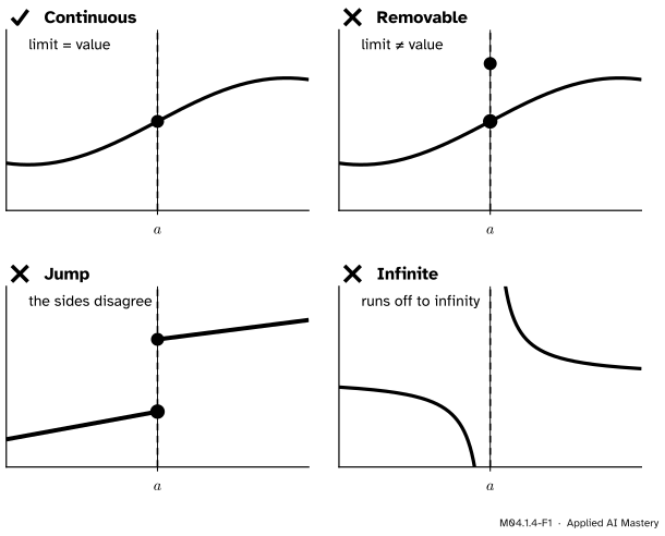
Continuity at \(a\), and three common ways to lose it. Removable: the curve heads to a height but the value is elsewhere, or missing. Jump: the two sides head to different heights. Infinite: the function runs off.
Each failure breaks a different link. A removable break has a limit that is not the value. A jump has no limit, because its one-sided limits differ. An infinite break has no finite limit at all.
Build it up
Step 1. Removable. The slope formula \({(x^2 - 1)/(x - 1)}\) of M04.1.1 has limit 2 at 1 but no value there. Define its value at 1 to be 2 and the break is gone, which is why it is called removable.
Step 2. Jump. The step function \(H\) has one-sided limits 0 and 1 at 0. No choice of \({H(0)}\) repairs that.
Step 3. Infinite.\({1/x}\) runs off to \({\pm\infty}\) at 0. Again, no value at 0 can repair it.
Step 4. What is continuous. Direct substitution (M04.1.2) says exactly that polynomials are continuous everywhere, and rational functions wherever their bottom is not 0. Sums, products and quotients of continuous functions are continuous, by the limit laws (a quotient wherever its bottom is not 0). We state, without proof, that compositions of continuous functions are continuous, and that \({\sin x}\), \({\cos x}\) and \({e^x}\) are continuous everywhere and \({\ln x}\) and \({\sqrt{x}}\) on their domains. So the sigmoid, built from \({e^{-z}}\) by adding and dividing, is continuous too.
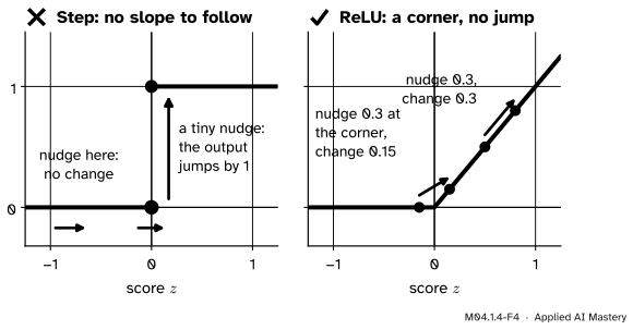
Step 5. ReLU against the step. ReLU is 0 to the left of 0 and \(z\) to the right. At 0 both sides head to 0, and the value is 0: continuous, with a corner. A nudge of size \(\Delta\) to its input changes its output by at most \(\Delta\). If both inputs are positive the change is exactly \(\Delta\); if both are negative it is 0; and across 0 it is the positive input, which is less than \(\Delta\). The step obeys no such rule: a nudge from \({-0.001}\) to \({0.001}\) changes its output by 1.
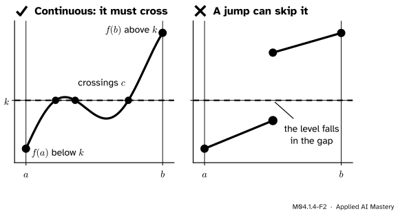
Step 6. Crossing a level. Draw a continuous curve from a point below a horizontal line to a point above it. However it wanders, the pen must cross the line somewhere. A jump could skip it.
M04.1.4-F2
The intermediate value theorem in a picture. Left: a continuous function that starts below the level \(k\) and ends above it crosses \(k\) at least once (here three times). Right: with a jump, the level can fall in the gap and never be reached.
The formal statement
NoteDefinition: continuity
A function \(f\) is continuous at \(a\) if three things hold:
\({f(a)}\) is defined;
\({\lim_{x \to a} f(x)}\) exists;
\({\lim_{x \to a} f(x) = f(a)}\).
It is continuous on an interval \({[a, b]}\) if it is continuous at every point inside, and at each end the one-sided limit from inside equals the value. A point where \(f\) is not continuous is a discontinuity: removable if the limit exists, a jump if both one-sided limits exist but differ, and infinite if a one-sided limit is \({\pm\infty}\).
These three are the common kinds, not the only ones. \({\sin(\pi / x)}\) of M04.1.1, whatever value it is given at 0, swings ever faster near 0 and has no one-sided limits there at all.
In the language of the game, continuity at \(a\) says: for every tolerance \(\varepsilon\) there is a window \(\delta\) such that every \(x\) within \(\delta\) of \(a\), now including \(a\) itself, has \({f(x)}\) within \(\varepsilon\) of \({f(a)}\). Small changes of input give small changes of output, which is exactly what training by small nudges relies on.
NoteThe intermediate value theorem
Let \(f\) be continuous on \({[a, b]}\), and let \(k\) be any number between \({f(a)}\) and \({f(b)}\). Then there is at least one \(c\) in \({[a, b]}\) with \({f(c) = k}\).
The theorem says that a solution exists, not where it is or how many there are. Its most used form takes \({k = 0}\): if \({f(a)}\) and \({f(b)}\) have opposite signs, \(f\) has a zero between them.
Bisection turns that form into a method. Start with \({[a, b]}\) where the signs differ, and repeat:
Find the midpoint \({m = (a + b)/2}\) and compute \({f(m)}\).
If \({f(m)}\) has the sign of \({f(a)}\), the change of sign is in \({[m, b]}\): replace \(a\) by \(m\). Otherwise it is in \({[a, m]}\): replace \(b\) by \(m\).
Each round keeps a smaller interval where the signs still differ, so by the theorem it still holds a zero, and it is half as wide. After \(n\) rounds the width is \({(b - a)/2^n}\). To shrink an interval of width 1 below \({10^{-6}}\) needs \({2^n \geq 10^6}\), which first holds at \({n = 20}\), since \({2^{20} = 1{,}048{,}576}\).
Go deeper: why the intermediate value theorem is true
Bisection is the proof. Take \({f(a) < 0 < f(b)}\) and run it for ever, keeping \({f < 0}\) at the left end and \({f \geq 0}\) at the right end of every interval. The left ends never decrease, the right ends never increase, and the widths \({(b - a)/2^n}\) tend to 0, so both ends close in on a single number \(c\) (that a number is there to close in on is completeness again, the property of the real numbers met in M04.1.3). By continuity, \({f(\text{left ends})}\) tends to \({f(c)}\), and each of those values is negative, so \({f(c) \leq 0}\). The right ends give \({f(c) \geq 0}\). So \({f(c) = 0}\). Any other level \(k\) comes down to this case: run the same argument on \({f(x) - k}\), or on \({k - f(x)}\) if \(f\) starts above \(k\).
Worked example
Find \({\sqrt{2}}\) by bisection on \({[1, 2]}\).
\({\sqrt{2}}\) is the positive zero of \({f(x) = x^2 - 2}\), a polynomial, so \(f\) is continuous. At the ends \({f(1) = -1 < 0}\) and \({f(2) = 2 > 0}\), so by the theorem a zero lies in \({[1, 2]}\).
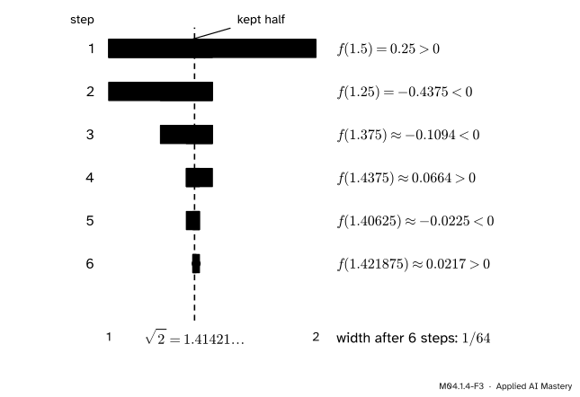
Step 1: \({m = 1.5}\), \({f(m) = 0.25 > 0}\). The sign change is on the left: keep \({[1, 1.5]}\).
After six steps \({\sqrt{2}}\) is pinned in an interval of width \({1/64 = 0.015625}\). The true value, 1.41421356, is inside.
M04.1.4-F3
Six steps of bisection for \({x^2 - 2}\). Each row halves the interval and keeps the half where the sign changes; the dashed line, \({\sqrt{2}}\), stays inside every kept half.
Bisection is slow but certain. It needs only the sign of \({f}\), never a formula for a solution, so it works for any continuous function you can evaluate.
Code
Bisection from scratch. The loop keeps halving until the interval is narrower than tol.
import mathdef bisection(f, a, b, tol=1e-6):"""A zero of f in [a, b], where f(a) and f(b) have opposite signs. Returns the midpoint of the last interval and the number of halvings.""" fa = f(a)if fa * f(b) >0:raiseValueError("f(a) and f(b) must have opposite signs") steps =0while b - a > tol: m = (a + b) /2 fm = f(m)if fm ==0:return m, steps +1if (fm <0) == (fa <0): # same sign as f(a): the zero is in [m, b] a, fa = m, fmelse: # the zero is in [a, m] b = m steps +=1return (a + b) /2, stepsroot, steps = bisection(lambda x: x**2-2, 1, 2)print(f"after {steps} halvings: {root:.8f} math.sqrt(2) = {math.sqrt(2):.8f}")print(f"error: {abs(root - math.sqrt(2)):.1e}")
after 20 halvings: 1.41421366   math.sqrt(2) = 1.41421356
error: 9.5e-08
Twenty halvings, as the count \({2^{20} \geq 10^6}\) predicted, and the midpoint is within \({2^{-21} \approx 4.8 \times 10^{-7}}\) of \({\sqrt{2}}\). SciPy’s bisect takes the same arguments: a function and an interval whose ends have opposite signs. Its default tolerance is \({2 \times 10^{-12}}\).
The same code finds a decision threshold. A classifier that predicts “yes” when the probability \({\sigma(z)}\) is at least \({\tau = 0.9}\) needs the score \(c\) with \({\sigma(c) = 0.9}\), which is \({c = \ln(\tau/(1 - \tau)) = \ln 9}\) (NOTATION.md).
This module’s interactive, the limit window, lives in lesson M04.1.1. The curve\({y = x^2}\) is continuous at 1: its limit there is 1, which is also its value. The jump is a jump discontinuity: once \({\varepsilon \leq 1}\) no window works. The hole is a removable one: some window always works, but the function has no value at 1 until we define one.
Pitfalls
M04.1.4-F4
Wrong beside right. Left: nudging the score of a step either changes nothing or flips the output by a whole 1, so there is no gradual change to follow. Right: ReLU has a corner but no jump, so a nudge always gives a change no bigger than itself.
“ReLU has a corner, so it is as bad as the step.”
The corner is not a break. ReLU is continuous, so small nudges give small changes, and those changes can be followed. The step jumps, so its output is flat almost everywhere and leaps at 0: there is nothing to follow. What the corner does affect is the slope at 0 itself, which has two one-sided values (M04.2.3).
“Continuous means smooth.”
Continuous means no breaks. \({\abs{x}}\) and ReLU are continuous everywhere, corners and all. Smoothness, having a slope everywhere, is a stronger property that M04.2 defines.
“If \({f(a)}\) and \({f(b)}\) have the same sign, there is no zero between them.”
\({x^2 - 1}\) is 3 at both \({-2}\) and 2, yet it is 0 at \({-1}\) and at 1. The theorem is silent when the signs agree; it never says that a zero is missing. Bisection needs a sign change to start.
“A change of sign always means a zero in between.”
Only for a continuous function. \({1/x}\) is \({-1}\) at \({-1}\) and \({\tfrac12}\) at 2, yet it is never 0. Run bisection on \({[-1, 2]}\) anyway and it closes in on \({x = 0}\), the asymptote, where \({1/x}\) has no value at all. Check continuity before you trust the answer.
Check yourself
Recall
1. What three conditions make \(f\) continuous at \(a\)?
Show answer
\({f(a)}\) is defined, \({\lim_{x \to a} f(x)}\) exists, and the two are equal.
2. Name the three kinds of discontinuity of this lesson, with an example of each.
Show answer
Removable, as \({(x^2 - 1)/(x - 1)}\) at 1; jump, as the step function at 0; infinite, as \({1/x}\) at 0.
3. Is ReLU continuous at 0? Why?
Show answer
Yes. Both one-sided limits are 0, and \({\max(0, 0) = 0}\). It has a corner there, not a break.
4. State the intermediate value theorem.
Show answer
If \(f\) is continuous on \({[a, b]}\) and \(k\) lies between \({f(a)}\) and \({f(b)}\), then \({f(c) = k}\) for at least one \(c\) in \({[a, b]}\).
5. Bisection starts on an interval of width 1. How wide is the interval after 10 steps?
Show answer
\({1/2^{10} = 1/1024}\), a little under 0.001.
Exercises
1.★ Classify each discontinuity, and say whether it can be removed: \({(x^2 - 4)/(x - 2)}\) at 2; the step function at 0; \({1/(x - 3)}\) at 3.
Show solution
\({(x^2 - 4)/(x - 2) = x + 2}\) for \({x \neq 2}\), so its limit at 2 is 4 but it has no value there: removable, by defining the value at 2 to be 4. The step has one-sided limits 0 and 1 at 0: a jump, which no value repairs. \({1/(x - 3)}\) runs to \({+\infty}\) from the right of 3 and to \({-\infty}\) from the left: infinite, which no value repairs either.
2.★★ Show that \({\sigma(z) = 0.9}\) has a solution between 0 and 3, and take three steps of bisection by hand.
Show solution
\(\sigma\) is continuous, \({\sigma(0) = 0.5 < 0.9}\) and \({\sigma(3) \approx 0.9526 > 0.9}\), so by the theorem some \(c\) in \({[0, 3]}\) has \({\sigma(c) = 0.9}\). Bisect the sign of \({\sigma(z) - 0.9}\):
The exact solution, \({c = \ln 9 \approx 2.1972}\), lies in \({[1.875, 2.25]}\), as it must.
3.★★★ Show that \({x^3 - 3x = 1}\) has three solutions, and say how many bisection steps pin each one in an interval of width at most 0.001.
Show solution
Let \({g(x) = x^3 - 3x}\), the course’s cubic, a polynomial and so continuous. Its values at the whole numbers from \({-2}\) to 2 are \({g(-2) = -2}\), \({g(-1) = 2}\), \({g(0) = 0}\), \({g(1) = -2}\) and \({g(2) = 2}\).
The level 1 lies between \({g(-2)}\) and \({g(-1)}\), between \({g(-1)}\) and \({g(0)}\), and between \({g(1)}\) and \({g(2)}\). By the theorem there is a solution in each of \({[-2, -1]}\), \({[-1, 0]}\) and \({[1, 2]}\), three intervals that do not overlap. A cubic equation has at most three solutions (M01.9.4), so these are all of them. Each interval has width 1. After 9 steps the width is \({1/512}\), still more than 0.001; after 10 it is \({1/1024}\), below 0.001. So 10 steps pin each one. The solutions are about \({-1.5321}\), \({-0.3473}\) and \({1.8794}\).
Summary card
Continuous means the value is where the graph is heading.
M04.1.4-F1
One way to hold, three common ways to break.
Continuity at \(a\).\({\lim_{x \to a} f(x)}\) exists and equals \({f(a)}\).
Breaks. Removable (limit not the value), jump (sides differ), infinite (runs off).
ReLU is continuous with a corner; the step jumps.
Intermediate values. Continuous on \({[a, b]}\) with a sign change means a zero inside; bisection finds it, halving the interval at every step.
Sources and next steps
Sources. Each was opened and checked against this lesson on 12 November 2026.
Gilbert Strang and Edwin Herman, Calculus Volume 1 (OpenStax), Section 2.4, Continuity: continuity at a point by three conditions; removable, jump and infinite discontinuities; the continuity of polynomials and rational functions on their domains (Theorem 2.8), of compositions (Theorem 2.9) and of the trigonometric functions (Theorem 2.10); and the intermediate value theorem (Theorem 2.11).
Matthew Boelkins, Active Calculus (single variable), Section 1.7, Limits, continuity, and differentiability: left-hand and right-hand limits (Definition 1.7.1), a function with a jump at \({a = 1}\) that has no limit there, and continuity at a point (Definition 1.7.4).
Michael Nielsen, Neural Networks and Deep Learning, Chapter 1, “Sigmoid neurons”: a small change in the weights or bias of a perceptron can flip its output from 0 to 1, while the smoothness of \(\sigma\) makes small changes in the weights produce small changes in the output.
Qingkai Kong, Timmy Siauw and Alexandre Bayen, Python Programming and Numerical Methods, Section 19.3, Bisection method: the intermediate value theorem as the reason bisection works, and \({\sqrt{2}}\) found as the zero of \({x^2 - 2}\).
SciPy reference, scipy.optimize.bisect (version 1.18): \(f\) must be continuous and \({f(a)}\) and \({f(b)}\) must have opposite signs; the default absolute tolerance xtol is \({2 \times 10^{-12}}\).
Next. Module M04.2, The derivative as slope and rate, takes the slope of a curve at a point as a limit, the question this module began with.