seaborn maps the columns of a long table to x, y and hue. Draw temperature by day coloured by station as a Matplotlib loop over groups, then in one seaborn call; meet axes-level and figure-level functions on iris, and see that barplot and lineplot compute a mean before they draw.
P02.8.4L1 Core25 minIn review (what this means)
The maths and code on this page are checked by automated tests on every change, but an independent reader has not signed it off yet. Spot a mistake or a confusing step? Tell us.
Explain how seaborn assigns the columns of a long table to the x, y and hue of a plot.
Write the Matplotlib loop over groupby groups that one seaborn call with hue replaces, and check that both draw the same points.
Tell axes-level functions (scatterplot, lineplot, histplot, boxplot) from figure-level ones (relplot, displot, catplot), and say what each returns.
Compute by hand the group means that barplot and lineplot draw, and state the error bar that is shown or switch it off with errorbar=None.
The question
The table readings has one row per reading: day, station, temperature and sky. In the last lesson, colouring the points by station took a loop and a legend. Can a whole long table be drawn in one line, and what does that one line quietly compute on the way?
From the last lesson
1. What does plt.subplots(1, 3) return as its second value, and of what shape?
Show answer
A NumPy array of three Axes, of shape (3,).
2. What does sharey=True do?
Show answer
It gives every panel the same y limits, fitted to all the panels’ data, so that a height means the same value everywhere.
Intuition
A long (or tidy) table has one row per observation and one column per variable (Wickham 2014, met in P02.5.3). readings is long: twelve rows, columns day, station, temp and sky. In such a table every column is a variable that a plot can show.
seaborn is a plotting library built on Matplotlib. You hand it the table and give each column a job: this column across (x), that one up (y), this one as colour (hue). seaborn does the splitting, the colouring and the legend.
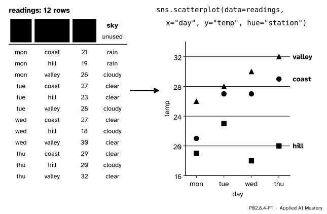
P02.8.4-F1
seaborn’s idea in one picture: columns of a long table become the jobs of the plot. Three columns are used; sky is free for another plot.
The colours and the legend were the loop’s work before. Now they are the table’s: because station is a column, seaborn can split the rows by it, just as groupby does.
Build it up
Step 1. The table. Build readings from temps with two loops, one row per day and station, and add the sky column. Twelve rows, ordered by day and then station.
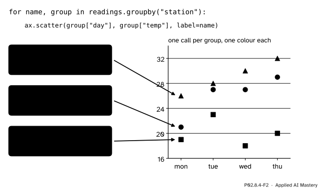
Step 2. The loop, by hand. Split the rows by station with groupby (P02.6) and call ax.scatter once per group, with label=name. Three calls give three colours, and ax.legend() collects the labels.
P02.8.4-F2
What hue replaces: a loop that splits the rows into groups and draws each group with its own call, colour and legend entry.
Step 3. One call.sns.scatterplot(data=readings, x="day", y="temp", hue="station", ax=ax) draws the same twelve points. The values of station become the colours, in the order they first appear, and the column name becomes the legend’s title.
Step 4. It is still Matplotlib. The call returns the Axes it drew on, so everything from the earlier lessons works on it: ax.set_ylim, ax.set_title, ax.axhline.
Step 5. A computed plot.sns.barplot(data=readings, x="sky", y="temp") does not draw rows. It groups the rows by sky, takes the mean of each group, and draws one bar per mean. seaborn computes before it draws.
The formal statement
NoteDefinition: seaborn’s two kinds of function
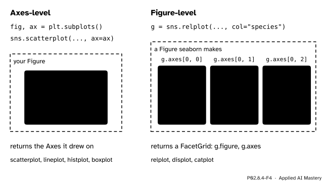
An axes-level function, such as scatterplot, lineplot, histplot or boxplot, draws onto one Matplotlib Axes, the one passed as ax= (or the current one), and returns that Axes.
A figure-level function, relplot, displot or catplot, makes its own Figure, can lay out one panel per value of a column with col= (and row=), and returns a FacetGrid, which holds the Figure (g.figure) and an array of Axes (g.axes).
In both, data= takes a long table and x=, y= and hue= take column names.
P02.8.4-F4
Axes-level functions draw where you tell them. Figure-level functions own their figure and can split it into panels.
The axes-level functions fit the explicit style of this module: make the Figure and Axes yourself, then let seaborn draw on one. The figure-level ones save the layout work of P02.8.3 when you want one panel per group.
What the computing plots compute. For a column \(y\) grouped by a column \(x\), barplot and lineplot draw, for each value \(g\) of \(x\), the mean of the \(n_g\) readings in that group:
By default they also draw an error bar, errorbar=("ci", 95): a 95 per cent confidence interval for that mean, found by bootstrapping, which means resampling the group’s rows at random with replacement, a thousand times by default, and seeing how much the mean moves. Because it is random, the interval can differ slightly from run to run unless seed= is fixed. What such an interval means, and when it can be trusted, is P04.5; until then, say which error bar a chart shows, or pass errorbar=None to draw none.
Worked example
What does sns.barplot(data=readings, x="sky", y="temp", errorbar=None) draw?
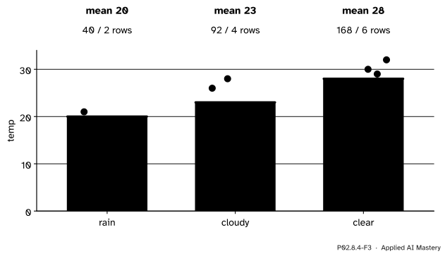
P02.8.4-F3
barplot groups the rows, computes each group’s mean and draws it as a bar. The dots, which barplot does not draw, are the readings it averaged.
Group the twelve rows by sky, in the order the values first appear in the table: rain (Monday), then cloudy (Monday), then clear (Tuesday).
rain: coast and hill on Monday, 21 and 19. Sum 40, two rows, mean \({40 / 2} = 20\).
cloudy: valley Monday 26, valley Tuesday 28, hill Wednesday 18, hill Thursday 20. Sum 92, four rows, mean \({92 / 4} = 23\).
clear: coast and hill Tuesday 27 and 23, coast and valley Wednesday 27 and 30, coast and valley Thursday 29 and 32. Sum 168, six rows, mean \({168 / 6} = 28\).
Check: \(2 + 4 + 6 = 12\) rows, and \(40 + 92 + 168 = 300 = {12 \times 25}\), the overall mean of 25. The chart has three bars, of heights 20, 23 and 28, in the order rain, cloudy, clear. These are the numbers of readings.groupby("sky")["temp"].mean() from P02.6.2, which lists them in sorted order instead: clear, cloudy, rain.
Code
The long table, built with two loops from temps.
import matplotlib.pyplot as pltimport numpy as npimport pandas as pdimport seaborn as snstemps = np.array([[21, 19, 26], [27, 23, 28], [27, 18, 30], [29, 20, 32]])days = ["mon", "tue", "wed", "thu"]stations = ["coast", "hill", "valley"]rows = []for i, day inenumerate(days):for j, station inenumerate(stations): rows.append({"day": day, "station": station, "temp": int(temps[i, j])})readings = pd.DataFrame(rows)readings["sky"] = ["rain", "rain", "cloudy", "clear", "clear", "cloudy","clear", "cloudy", "clear", "clear", "cloudy", "clear"]print(readings.head(4))print(readings.shape)
   day station  temp     sky
0  mon   coast    21    rain
1  mon    hill    19    rain
2  mon  valley    26  cloudy
3  tue   coast    27   clear
(12, 4)
The loop by hand: one scatter call per group, then the same plot from seaborn in one call.
fig, ax = plt.subplots(figsize=(5, 3))for name, group in readings.groupby("station"): ax.scatter(group["day"], group["temp"], label=name)ax.legend(title="station")by_hand =sorted(tuple(p) for c in ax.collections for p in c.get_offsets().tolist())print(len(ax.collections), "calls,", [t.get_text() for t in ax.get_legend().get_texts()])plt.close(fig)fig, ax = plt.subplots(figsize=(5, 3))returned = sns.scatterplot(data=readings, x="day", y="temp", hue="station", ax=ax)by_seaborn =sorted(tuple(p) for c in ax.collections for p in c.get_offsets().tolist())print(returned is ax, [t.get_text() for t in ax.get_legend().get_texts()])print("same points:", by_hand == by_seaborn)plt.close(fig)
seaborn computes before it draws. With errorbar=None, barplot draws the group means alone, and lineplot of temperature by day draws the mean of each day.
fig, ax = plt.subplots(figsize=(4, 3))sns.barplot(data=readings, x="sky", y="temp", errorbar=None, ax=ax)order = [label.get_text() for label in ax.get_xticklabels()]heights = [float(bar.get_height()) for bar in ax.patches]print(order, heights)plt.close(fig)fig, ax = plt.subplots(figsize=(4, 3))sns.lineplot(data=readings, x="day", y="temp", errorbar=None, ax=ax)print("day means:", ax.lines[0].get_ydata().tolist())plt.close(fig)print(readings.groupby("sky")["temp"].agg(["size", "sum", "mean"]))
['rain', 'cloudy', 'clear'] [20.0, 23.0, 28.0]
day means: [22.0, 26.0, 25.0, 27.0]
        size  sum  mean
sky
clear      6  168  28.0
cloudy     4   92  23.0
rain       2   40  20.0
The day means 22, 26, 25 and 27 are those of temps.mean(axis=1) in P02.2.2. Without errorbar=None, barplot adds an error bar to each bar; its ends come from random resampling, so only their number is checked here, not their values.
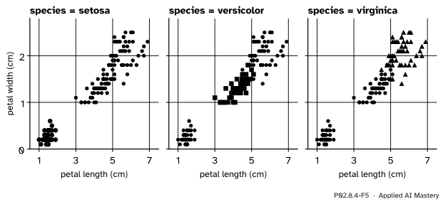
A figure-level function on real data: scikit-learn’s iris, 150 flowers of three species, one panel per species. relplot makes the Figure and returns a FacetGrid.
from sklearn.datasets import load_irisiris = load_iris(as_frame=True)flowers = iris.frame.copy()flowers["species"] = iris.target_names[iris.target]g = sns.relplot(data=flowers, x="petal length (cm)", y="petal width (cm)", hue="species", col="species", height=3)print(type(g).__name__, g.axes.shape)print([ax.get_title() for ax in g.axes.flat])plt.close(g.figure)
The relplot call above, drawn in the site’s style. One panel per value of col: setosa stands apart on petal size, and versicolor and virginica overlap only a little, which is why iris is a first classification problem in machine learning.
Explore
This module’s interactive, Figure anatomy, is in lesson P02.8.1. Every part it switches on is a part that seaborn also makes for you: its axis labels come from the column names, its legend from hue. Because seaborn returns ordinary Axes, any of those parts can still be changed afterwards with the calls the interactive shows.
Pitfalls
P02.8.4-F6
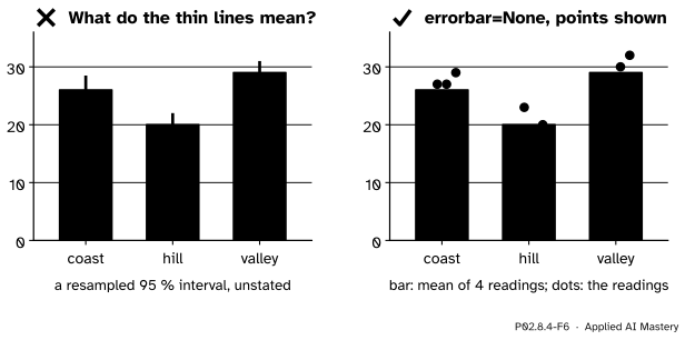
Wrong beside right. barplot’s default error bars are a random-resampling interval that the chart never names; the right-hand chart says what it shows and shows the readings themselves.
“A seaborn bar is a value from my table.”
It is a summary of several rows, by default their mean, and the thin line on it is an error bar that you did not ask for. Say what the bar and the line are, in the caption or the axis label, or draw them yourself: errorbar=None, and the points on top with sns.stripplot or ax.scatter. With four readings per bar, the readings are more honest than any interval.
“seaborn takes any table.”
It wants a long table, one row per observation, so that x, y and hue can each name a column. The wide table of P02.4, one column per station, has no station column to colour by. Melt it first (wide.melt(...), P02.5.3), then plot.
“relplot(...) returns an Axes like scatterplot(...) does.”
Figure-level functions return a FacetGrid. Calling g.set_title(...) on it fails; reach the Axes through g.axes (an array, as in P02.8.3) and the Figure through g.figure, or use an axes-level function with ax= when you need one Axes in a layout of your own.
Check yourself
Recall
1. What makes a table long, or tidy?
Show answer
Each variable is a column and each observation is a row: one row per reading.
2. What does hue="station" do in sns.scatterplot?
Show answer
It splits the rows by the values of the station column and gives each group its own colour and legend entry, the work of a groupby loop.
3. What do an axes-level and a figure-level function return?
Show answer
An axes-level function returns the Matplotlib Axes it drew on; a figure-level function returns a FacetGrid, holding the Figure and an array of Axes.
4. What heights does sns.barplot(data=readings, x="sky", y="temp") draw, and in what order?
Show answer
The group means 20, 23 and 28, in the order the values first appear: rain, cloudy, clear.
5. What is barplot’s default error bar, and how do you remove it?
Show answer
A 95 per cent confidence interval for the mean, found by bootstrap resampling (errorbar=("ci", 95)); errorbar=None removes it.
Exercises
1.★ By hand, what does sns.barplot(data=readings, x="station", y="temp", errorbar=None) draw? Check the overall mean from the bars.
Show solution
Three bars in the order the stations first appear, coast, hill, valley, with heights equal to the station means: \({(21 + 27 + 27 + 29) / 4} = 26\), \({(19 + 23 + 18 + 20) / 4} = 20\) and \({(26 + 28 + 30 + 32) / 4} = 29\). Each group has four rows, so the overall mean is the mean of the bars: \({(26 + 20 + 29) / 3} = 25\).
2.★★ Why is the mean of the three sky bars, \({(20 + 23 + 28) / 3}\), not the overall mean of 25? Compute the right weighted mean from the bars.
Show solution
\({(20 + 23 + 28) / 3} = {71 / 3} \approx 23.67\). The groups have different sizes, 2, 4 and 6 rows, so each bar must count as many times as it has rows:
A chart of group means hides the group sizes, which is one more reason to show the counts or the points.
3.★★★ Write the loop that sns.lineplot(data=readings, x="day", y="temp", errorbar=None) replaces, without seaborn, and say which numbers it draws.
Show solution
means = readings.groupby("day", sort=False)["temp"].mean()fig, ax = plt.subplots()ax.plot(means.index, means.to_numpy(), marker="o")
lineplot groups the rows by day (here three readings per day), takes each group’s mean and joins the means in order: 22, 26, 25 and 27 for Monday to Thursday, the day means of temps.mean(axis=1). sort=False keeps the days in table order; sorted alphabetically they would run mon, thu, tue, wed and the line would zigzag through time.
Summary card
seaborn turns the columns of a long table into the jobs of a plot, and computes before it draws.
Axes-level: scatterplot, lineplot, histplot, boxplot. Figure-level, with col=: relplot, displot, catplot, returning a FacetGrid.
barplot and lineplot draw group means; by sky they are 20, 23, 28.
The default error bar is a bootstrap 95 per cent interval: state it, or errorbar=None.
Sources and next steps
Sources. Each was opened and checked against this lesson on 15 November 2026.
seaborn developers, Overview of seaborn plotting functions, seaborn 0.13.2. Section Figure-level vs. axes-level functions: axes-level functions plot onto one Matplotlib Axes, which is their return value, and accept ax=; relplot, displot and catplot are figure-level and return a FacetGrid.
seaborn developers, Data structures accepted by seaborn, seaborn 0.13.2: a long-form table has each variable as a column and each observation as a row, and its columns are given roles by assigning their names to x, y and hue.
seaborn developers, seaborn.barplot and seaborn.lineplot, seaborn 0.13.2: defaults estimator='mean', errorbar=('ci', 95) and n_boot=1000, a seed for reproducible bootstrapping, and None to hide the error bar; lineplot aggregates repeated \(x\) values to show the mean and a 95 per cent confidence interval.
seaborn developers, Statistical estimation and error bars, seaborn 0.13.2: errorbar="ci" draws a 95 per cent confidence interval, found by bootstrapping, in which the dataset is resampled at random with replacement.
Hadley Wickham, Tidy Data, Journal of Statistical Software 59(10), 2014: in tidy data each variable is a column, each observation is a row, and each type of observational unit is a table.
Next.P02.9 Reproducible notebooks puts the loading, cleaning, summarising and plotting of this course into a notebook that anyone can rerun. The grammar of graphics behind seaborn is P04.2, choosing a chart is P04.3, and showing uncertainty honestly is P04.5.