\( \newcommand{\vect}[1]{\boldsymbol{\mathbf{#1}}} \newcommand{\mat}[1]{\boldsymbol{\mathbf{#1}}} \newcommand{\R}{\mathbb{R}} \newcommand{\E}{\mathbb{E}} \newcommand{\Prob}{\mathbb{P}} \newcommand{\T}{^{\top}} \newcommand{\norm}[1]{\lVert #1 \rVert} \newcommand{\abs}[1]{\lvert #1 \rvert} \newcommand{\ihat}{\mkern1mu\hat{\boldsymbol{\imath}}\mkern2mu} \newcommand{\jhat}{\mkern1mu\hat{\boldsymbol{\jmath}}\mkern2mu} \newcommand{\pd}[2]{\frac{\partial #1}{\partial #2}} \newcommand{\argmax}{\operatorname*{arg\,max}} \newcommand{\argmin}{\operatorname*{arg\,min}} \newcommand{\cdata}[1]{\class{c-data}{#1}} \newcommand{\cmodel}[1]{\class{c-model}{#1}} \newcommand{\ctruth}[1]{\class{c-truth}{#1}} \newcommand{\cgrad}[1]{\class{c-grad}{#1}} \newcommand{\closs}[1]{\class{c-loss}{#1}} \newcommand{\cparam}[1]{\class{c-param}{#1}} \newcommand{\csecond}[1]{\class{c-second}{#1}} \renewcommand{\,}{\mkern3mu} \)

Positions and slices

Read one entry, a row, a column or a block of a 2-D array with one bracket: a position or a start:stop:step slice per axis. See why an integer drops its axis while a slice keeps it, and how None adds an axis ready for broadcasting.

P02.3.1L1 Core25 min

In review (what this means)

The maths and code on this page are checked by automated tests on every change, but an independent reader has not signed it off yet. Spot a mistake or a confusing step? Tell us.

Before this lesson: P01.6 Lists, tuples, dictionaries and sets P02.1 Arrays, shapes and data types P02.2 Broadcasting and vectorization

What you will be able to do

• Read an entry, a row, a column and a block of a 2-D array with one index per axis, using positions from the front and from the back.
• Predict the rows a start:stop:step slice keeps, and count them with the ceiling formula.
• Predict the shape of a result: an integer drops its axis, a slice keeps it, and None adds one of size 1.
• Cut the same block out of nested lists with a comprehension and out of an array with one slice expression.

The question

A dataset arrives as one array: one row per example, one column per feature, and the labels in the last column. To train a model you need the features without the labels, one column to look at, the first few rows as a batch. Each of those is one short expression in square brackets. But why does temps[:, 0] come out with shape (4,) while temps[:, 0:1] has shape (4, 1), and why does that difference decide whether the next line of code works?

Intuition

This module works with the course’s running array. It holds noon temperatures, in degrees Celsius, at three weather stations (coast, hill and valley) on four days, Monday 3 to Thursday 6 March 2025. The numbers are invented for teaching. Rows are days and columns are stations:

import numpy as np

temps = np.array([[21, 19, 26],
                  [27, 23, 28],
                  [27, 18, 30],
                  [29, 20, 32]])
print(temps.shape)

(4, 3)

An index into a 2-D array names something along each axis, separated by a comma: first the rows (axis 0), then the columns (axis 1). For each axis you give either a single position, which picks one row or one column, or a slice, which keeps a run of them. Lesson P01.6.1 drew a slice of a list as two cuts between the slots. A grid has cuts between its rows and cuts between its columns, and a slice on each axis cuts out a block.

P02.3.1-F1

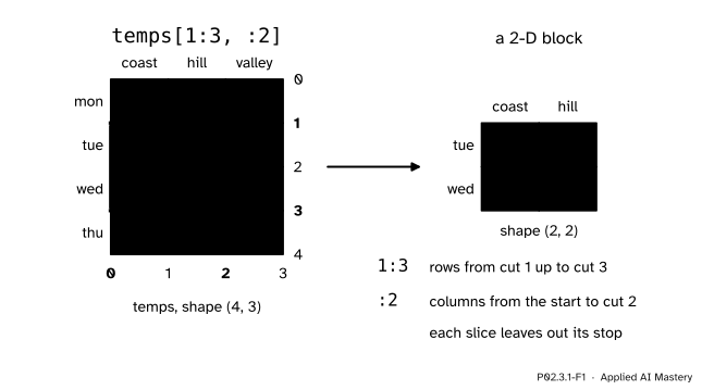
temps[1:3, :2] cuts the grid twice on each axis and keeps what lies inside: Tuesday and Wednesday at the coast and on the hill. The result is a new 2-D array, numbered from 0 again.

Reading the index from left to right: rows from cut 1 up to cut 3, so Tuesday and Wednesday; columns from the start up to cut 2, so coast and hill. The stop is never included, just as for lists.

Build it up

Step 1. One entry. Two positions name one cell. temps[1, 2] is Tuesday at the valley, 28. With nested lists the same cell takes two look-ups, rows[1][2]: first the inner list, then the item.

Step 2. A row. One position and nothing for the columns gives a whole row. temps[1] is Tuesday, [27, 23, 28]. An axis you do not mention is taken whole, so temps[1] means temps[1, :].

Step 3. A column. A colon on its own is the slice from the start to the end: the whole axis. So temps[:, 0] keeps every row and picks column 0, the coast readings [21, 27, 27, 29]. Nested lists have no way to say “every row” in one look-up; they need a comprehension, [row[0] for row in rows].

Step 4. A block. A slice on both axes keeps a rectangle, as in the anchor figure.

P02.3.1-F2

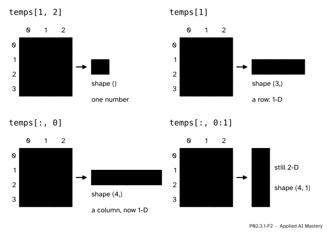
An entry, a row, a column and a column that keeps its axis. Look at the shapes: the integer 0 in temps[:, 0] removes the column axis, so the coast readings come out flat, while the slice 0:1 keeps the axis with length 1.

Step 5. Counting from the back, and steps. A negative position counts from the end, so temps[-1] is Thursday and temps[-1, -1] is 32. A slice may carry a third number, the step: temps[::2] keeps every second day starting at Monday, so Monday and Wednesday, and temps[::-1] walks backwards and gives the days in reverse order.

Step 6. Adding an axis. Writing None inside an index adds a new axis of length 1 at that place. The coast readings col = temps[:, 0] have shape (4,); col[:, None] is the same four numbers as a column of shape (4, 1), and col[None, :] is a row of shape (1, 4). NumPy also calls None here by the name np.newaxis. This is the third way, after keepdims=True and reshape(4, 1) in lesson P02.2.4, to turn a 1-D array into a column that broadcasts across the rows.

The formal statement

NoteDefinition: basic indexing

Let a be an array whose axis has length \(n\). On that axis an index is one of three things.

• An integer \(i\) with \({-n \le i < n}\). A negative \(i\) means position \({n + i}\). It picks one position and removes the axis from the result. Any other integer raises IndexError.
• A slice start:stop:step, with a step that is not 0. With a positive step it keeps the positions start, start + step, start + 2*step and so on, as long as they are below stop. A missing start means 0, a missing stop means \(n\), a missing step means 1, negative bounds count from the back, and bounds beyond the ends are moved to the ends. A negative step walks towards smaller positions, and then the missing start and stop mean “from the last” and “through the first”. A slice keeps the axis, with the number of positions it kept as its new length.
• None (also called np.newaxis) adds an axis of length 1 and uses up no axis of a.

Axes that the index does not mention are taken whole, as if written :.

The shape of the result. Go through the index from left to right. Each slice gives one axis of the result, as long as the number of positions it kept. Each None gives an axis of length 1. Each integer gives nothing. So temps[1:3, :2] has shape (2, 2), temps[1, :2] has shape (2,), temps[1:2, :2] has shape (1, 2), and temps[1, 2] has shape (), a single number.

How many positions a slice keeps. Take a positive step \(k\) and bounds already moved into range, \({0 \le \text{start} \le \text{stop} \le n}\). The kept positions are \({\text{start} + mk}\) for \({m = 0, 1, 2, \dots}\) as long as

\[ \text{start} + m\,k < \text{stop}. \]

Subtract start and divide by \(k\), which is positive, so the inequality keeps its direction:

\[ m < \frac{\text{stop} - \text{start}}{k}. \]

The whole numbers \(m\) from 0 that satisfy this are \({0, 1, \dots, M - 1}\), where \(M\) is the smallest whole number at least as large as the fraction. That is the fraction rounded up, its ceiling:

\[ \text{count} = \left\lceil \frac{\text{stop} - \text{start}}{k} \right\rceil . \]

For temps[1::2] the start is 1, the stop is 4 and the step is 2, so the count is the ceiling of 3/2, which is 2: Tuesday and Thursday. With step 1 the formula gives stop minus start, the rule for lists in P01.6.1.

P02.3.1-F3

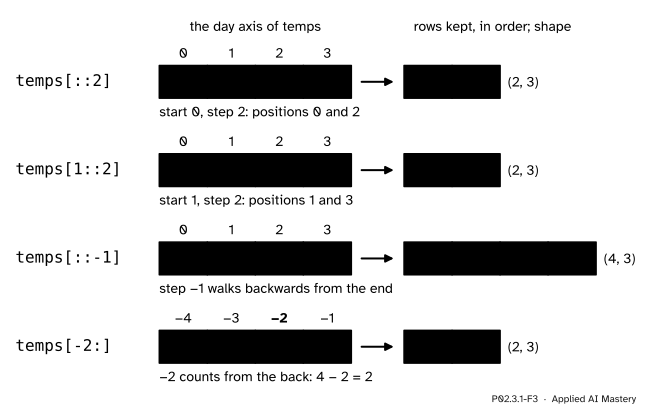
Start, stop and step along the day axis. Each slice keeps whole rows, so every result still has three columns; only the first axis changes length.

Go deeper: the ceiling written with whole-number division

Python has no ceiling for whole numbers, but floor division does the job: for positive \(k\), \({\lceil a / k \rceil}\) equals (a + k - 1) // k. Write \({a = qk + r}\) with \({0 \le r < k}\). If \({r = 0}\), both sides are \(q\), because adding \({k - 1}\) stays below the next multiple of \(k\). If \({r > 0}\), the ceiling is \({q + 1}\), and \({a + k - 1 = (q + 1)k + (r - 1)}\) with \({0 \le r - 1 < k}\), so the floor division also gives \({q + 1}\). Python’s own len(range(start, stop, step)) uses the same count, and a slice keeps exactly the positions of that range.

Worked example

Cut out Tuesday and Wednesday at the coast and on the hill, first from nested lists, then from the array, and predict the shape before running anything.

Nested lists. rows is a list of four inner lists, one per day. A list slice works on one level at a time, so the job takes two steps.

1. rows[1:3] keeps the inner lists at positions 1 and 2: [[27, 23, 28], [27, 18, 30]].
2. Each of those still has three readings. Cut each one with row[:2], inside a comprehension: [row[:2] for row in rows[1:3]] is [[27, 23], [27, 18]].

The array. One index does both steps at once: temps[1:3, :2].

The shape. The row slice 1:3 keeps \({3 - 1 = 2}\) positions and the column slice :2 keeps \({2 - 0 = 2}\). Both are slices, so both axes stay, and the shape is (2, 2).

P02.3.1-F4

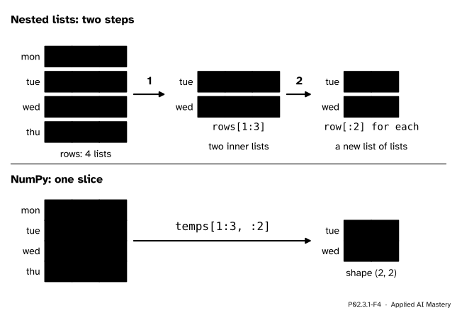
The worked example as a trace. With nested lists the rows are cut first and each row afterwards. The array takes both cuts in one index.

Change one character and the shape changes. temps[1:3, 0] has an integer for the columns, so that axis is dropped: the result is [27, 27] with shape (2,), Tuesday’s and Wednesday’s coast readings as a flat array.

Code

First the block from scratch, with nested lists, as a small function:

rows = [[21, 19, 26],
        [27, 23, 28],
        [27, 18, 30],
        [29, 20, 32]]

def block(rows, r0, r1, c0, c1):
    """Rows r0 up to r1 and columns c0 up to c1, each stop left out."""
    return [row[c0:c1] for row in rows[r0:r1]]

print(block(rows, 1, 3, 0, 2))
print([row[0] for row in rows])       # the coast column needs a loop

[[27, 23], [27, 18]]
[21, 27, 27, 29]

Then every selection of this lesson with one index each:

print(temps[1, 2], temps[1], temps[:, 0])
print(temps[1:3, :2])
print(temps[-1], temps[-1, -1])
print(temps[::2])
print(temps[:, 0].shape, temps[:, 0:1].shape, temps[:, 0][:, None].shape)

28 [27 23 28] [21 27 27 29]
[[27 23]
 [27 18]]
[29 20 32] 32
[[21 19 26]
 [27 18 30]]
(4,) (4, 1) (4, 1)

The count formula against NumPy, for every start, stop and step on an axis of four:

def count(start, stop, step):
    """Positions kept by start:stop:step (bounds in range, step positive)."""
    return max(0, (stop - start + step - 1) // step)

ok = all(count(s, e, k) == len(temps[s:e:k])
         for s in range(5) for e in range(5) for k in range(1, 5))
print(ok, count(1, 4, 2))

True 2

Where machine learning meets it: a table of examples with the label in its last column. Here the regression points of ML01, \({x = 1, 2, 3, 4}\) and \({y = 2, 3, 5, 6}\), sit side by side.

data = np.array([[1, 2],
                 [2, 3],
                 [3, 5],
                 [4, 6]])
X = data[:, :-1]          # every column but the last: stays 2-D
y = data[:, -1]           # the last column: 1-D
print(X.shape, y.shape)
for start in range(0, len(X), 2):
    print("batch", X[start:start + 2].ravel(), y[start:start + 2])

(4, 1) (4,)
batch [1 2] [2 3]
batch [3 4] [5 6]

Libraries such as scikit-learn expect exactly these shapes: a 2-D feature table X, one row per example, and a 1-D target y. The slice :-1 keeps the feature axis even when only one feature is left; the integer -1 drops it. The loop cuts the rows into the mini-batches of ML01.5.4.

Explore

This module’s interactive, the index explorer, lives in lesson P02.3.4, because its last button is about views. Its slice mode belongs to this lesson: set start, stop and step for rows and columns, and check each shape against the count formula before you look.

Pitfalls

P02.3.1-F5

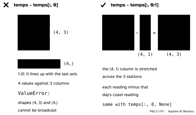
Wrong beside right. A column picked with an integer is 1-D, and broadcasting lines a 1-D array up with the last axis, here the three stations. Kept as a (4, 1) column, it stretches across them.

“temps[:, 0] is a column, so I can subtract it from every column.”

It holds a column’s values, but the integer removed the column axis: its shape is (4,). The broadcasting rule of P02.2.3 lines shapes up from the right, so its 4 meets the 3 stations and temps - temps[:, 0] raises ValueError. Keep the axis with temps[:, 0:1] or add it back with temps[:, 0, None].

“temps[:][0] is the same as temps[:, 0].”

Two pairs of brackets are two separate look-ups. temps[:] is the whole array, and [0] then takes its first row, Monday, [21, 19, 26]. Only one bracket with a comma, temps[:, 0], reaches the first column. For a single entry temps[1][2] happens to agree with temps[1, 2], which is why the habit survives.

“temps[1:3] gives rows 1, 2 and 3.”

A slice leaves out its stop. temps[1:3] keeps \({3 - 1 = 2}\) rows, Tuesday and Wednesday.

“A position past the end and a slice past the end both fail.”

Only the position does: temps[4] raises IndexError, because the array has rows 0 to 3. A slice moves its bounds into range, so temps[2:10] quietly keeps Wednesday and Thursday. That is convenient for the last, shorter mini-batch, and a trap when you expected an error.

Check yourself

Recall

1. What is temps[2, 1], and which day and station is it?

Show answer

18, the hill on Wednesday: row 2 is Wednesday and column 1 is the hill.

2. What are the shapes of temps[:, 1] and temps[:, 1:2]?

Show answer

(4,) and (4, 1). The integer drops the column axis; the slice keeps it with length 1.

3. Which days does temps[1::2] keep?

Show answer

Tuesday and Thursday: start at position 1 and step by 2, so positions 1 and 3.

4. What is temps[-1, 0]?

Show answer

29, Thursday at the coast. Position \({-1}\) on an axis of 4 is position \({4 - 1 = 3}\).

5. What does None do inside an index?

Show answer

It adds a new axis of length 1 at that place, without using up an axis of the array. So temps[:, 0][:, None] has shape (4, 1).

Exercises

1. ★ Write one index for each selection and give its shape: Monday’s three readings; the valley column; Wednesday and Thursday at the hill and the valley.

Show solution

Monday is temps[0], [21, 19, 26], shape (3,). The valley column is temps[:, 2] (or temps[:, -1]), [26, 28, 30, 32], shape (4,). Wednesday and Thursday at the hill and the valley is temps[2:, 1:], [[18, 30], [20, 32]], shape (2, 2): rows from cut 2 to the end, columns from cut 1 to the end.

2. ★★ How many rows does each keep, and which? temps[0:4:3], temps[1:], temps[3:1], temps[::-2]. Use the count formula where it applies.

Show solution

temps[0:4:3]: the ceiling of \({(4 - 0)/3}\) is 2, positions 0 and 3, Monday and Thursday.

temps[1:]: the stop is 4, so \({4 - 1 = 3}\) rows, Tuesday to Thursday.

temps[3:1]: the start is past the stop and the step is positive, so no rows at all. The result is an empty array of shape (0, 3), not an error.

temps[::-2]: a negative step starts from the last row and walks back two at a time, positions 3 and 1, so Thursday and then Tuesday, shape (2, 3).

3. ★★★ Write batches(X, size), which returns a list of consecutive row slices of X, each with size rows except perhaps the last. What shapes does it give for temps with size 3, and why does the last slice not fail?

Show solution

def batches(X, size):
    return [X[start:start + size] for start in range(0, len(X), size)]

For temps and size 3 the starts are 0 and 3, so the slices are temps[0:3], shape (3, 3), and temps[3:6], shape (1, 3). The second stop, 6, is past the end; a slice moves it back to 4, so the last batch is simply shorter. Both slices keep the row axis, so even a batch of one row is 2-D, which is what a model that expects a table of examples needs.

Summary card

One index per axis: a position picks, a slice cuts.

P02.3.1-F1

Two cuts on each axis keep a block.

• a[i, j] one entry; a[i] a row; a[:, j] a column; a[r0:r1, c0:c1] a block.
• Negative positions count from the back: \({-k}\) means \({n - k}\).
• start:stop:step keeps the ceiling of \({(\text{stop} - \text{start})/\text{step}}\) positions.
• An integer drops its axis, a slice keeps it, None adds one of length 1.

Sources and next steps

Sources. Each was opened and checked against this lesson on 15 November 2026.

• NumPy developers, Indexing on ndarrays, NumPy user guide, section Basic indexing, subsections Slicing and striding and Dimensional indexing tools: the slice i:j:k with its defaults and negative bounds and steps; an integer returns the same values as i:i+1 with one dimension fewer; newaxis is an alias for None and adds an axis of length one.
• Jake VanderPlas, Python Data Science Handbook, The Basics of NumPy Arrays, section Array Slicing: the pattern x[start:stop:step] with defaults 0, the size of the dimension and 1, and a negative step that swaps the defaults for start and stop.
• Python Software Foundation, The Python Tutorial, section 3.1.3, Lists: a list slice returns a new list, which is why nested lists need a comprehension to cut a column.

Next. P02.3.2 Boolean masks picks entries by a condition instead of by position: every reading above 27, or every day when the coast was warm.

This lesson unlocks

P02.3.2 Boolean masks

Your progress is saved in this browser only. No account, no tracking.