Place three panels by hand with fig.add_axes in fractions of the figure, then let plt.subplots do it: an array of Axes, one station per panel on a shared y axis. Mark values with axhline and annotate, label lines directly, and keep the styling in one function.
P02.8.3L1 Core25 minIn review (what this means)
The maths and code on this page are checked by automated tests on every change, but an independent reader has not signed it off yet. Spot a mistake or a confusing step? Tell us.
Compute the [left, bottom, width, height] rectangle of each panel by hand and place it with fig.add_axes.
Make a row of panels with plt.subplots(1, 3, sharey=True, layout=‘constrained’) and loop over the returned array of Axes.
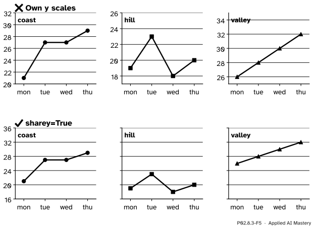
Explain why panels that are compared must share a y scale, and say which limits the shared scale gets.
Mark a value with ax.axhline and ax.annotate, label lines directly instead of with a legend, and collect styling in one function.
Draw a DataFrame onto an Axes you own with DataFrame.plot(ax=ax).
The question
You want to compare the three stations day by day. Three lines on one chart tangle; three separate charts can each look equally warm. How do you put several panels in one figure so that a reader compares them fairly, and without restyling each one by hand?
From the last lesson
1. With the edges 18, 22, 26, 30, 34, which bin holds the reading 30?
Show answer
The last bin, from 30 to 34: a value on an inner edge goes to the bin on its right.
2. Why must a bar chart’s axis start at zero?
Show answer
Because the eye compares the bars’ lengths, and a cut axis distorts the ratios between them.
Intuition
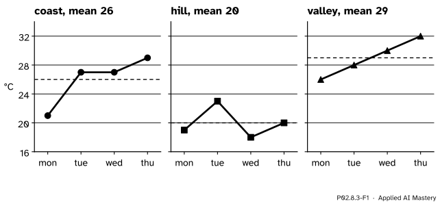
A Figure can hold any number of Axes. Give each station its own Axes, side by side, and the readings no longer cross each other. One rule makes the panels honest: they share one y scale, so that the same height means the same temperature in every panel.
P02.8.3-F1
One Figure, three Axes, one y scale. The hill station is visibly the coldest because a degree is the same height in every panel.
Two jobs come with several panels. The first is placing them: each Axes needs a rectangle inside the figure. The second is styling them all the same way, which is a loop, or better a function.
Build it up
Step 1. The canvas.plt.figure(figsize=(9, 3), dpi=100) makes a Figure 9 inches by 3 at 100 dots per inch: \({9 \times 100} = 900\) by \({3 \times 100} = 300\) pixels.
Step 2. One panel by hand.fig.add_axes([left, bottom, width, height]) adds an Axes whose rectangle is given in fractions of the figure, measured from the bottom-left corner. The rectangle [0.07, 0.15, 0.28, 0.75] starts 7 per cent of the way across and 15 per cent of the way up, and is 28 per cent wide and 75 per cent tall.
Step 3. Three by hand. Keep the bottom, width and height; move each panel right by its own width plus a gap of 0.03. The lefts are 0.07, 0.38 and 0.69, worked out in full below.
Step 4. Let Matplotlib do it.plt.subplots(1, 3) makes one row of three panels and returns them as a NumPy array of Axes. layout="constrained" sizes the gaps so that titles and tick labels do not collide, and sharey=True gives the panels one y scale.
Step 5. One panel per station. The array is indexed and looped like any array (P02.3): for ax, name, column in zip(axes, stations, temps.T) pairs each Axes with a station’s name and its column.
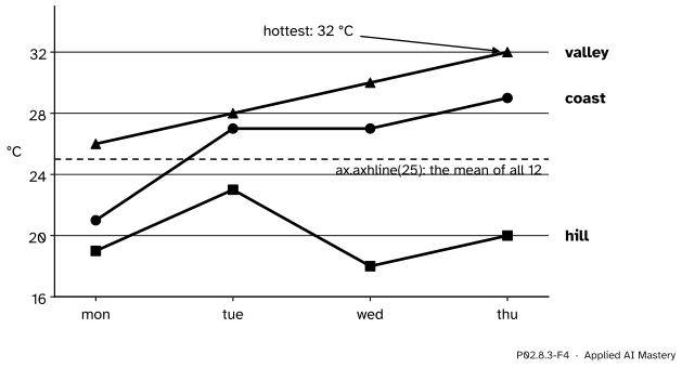
Step 6. Mark what matters.ax.axhline(25) draws a horizontal reference line across the Axes, here the mean of all twelve readings. ax.annotate(text, xy=point, xytext=place) writes a note with an arrow to a point. And ax.text can put each line’s name at its end, so that the reader does not have to match colours against a legend.
P02.8.3-F4
Direct labels at the ends of the lines, a reference line and an annotation, all on one Axes. No legend is needed.
Step 7. One style. Every panel needs the same title position, tick labels, limits and grid. Write those calls once, in a function style(ax, title), and call it for each Axes.
The formal statement
NoteDefinition: placing Axes in a Figure
fig.add_axes([left, bottom, width, height]) adds an Axes whose rectangle is given in fractions of the figure’s width and height, measured from its bottom-left corner.
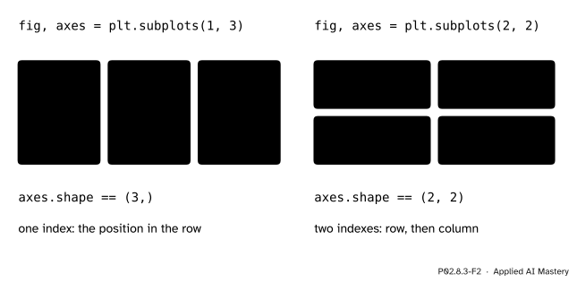
fig, axes = plt.subplots(nrows, ncols) makes a grid of Axes. With one row or one column, axes is a 1-D array of shape (n,); with several of each it is a 2-D array of shape (nrows, ncols), indexed row first; with one of each it is a single Axes.
sharey=True gives every panel the same y limits, chosen to fit the data of all panels; sharex=True does the same across.
P02.8.3-F2
The panels come back as an array with the grid’s shape. Rows come first, as in every NumPy shape.
Where the lefts come from. Take \(n\) panels of equal width \(w\) in one row, a margin \(m\) on the left, a margin \(r\) on the right and a gap \(g\) between neighbours. Across the figure, the pieces add up to the whole width, which is 1 in fractions:
\[
m + n\,w + (n - 1)\,g + r = 1.
\]
Solving for the width:
\[
w = \frac{1 - m - r - (n - 1)\,g}{n}.
\]
Panel \(k\), counting from 0, starts after the margin and after \(k\) panels and \(k\) gaps:
\[
\text{left}_k = m + k\,(w + g).
\]
Which limits the shared scale gets. Matplotlib pads the data range by 5 per cent at each end (P02.8.1). Shared across the three stations, the range runs from the lowest reading, 18, to the highest, 32, so it is 14 wide, the padding is \({0.05 \times 14} = 0.7\), and every panel shows 17.3 to 32.7. Each panel on its own would hug its own data instead: the hill alone, 18 to 23, would fill the same height as the valley alone, 26 to 32.
Worked example
Place three panels in a 900 by 300 pixel figure: a left margin of 0.07, a right margin of 0.03, gaps of 0.03, a bottom of 0.15 and a height of 0.75.
P02.8.3-F3
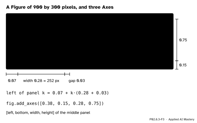
Three rectangles worked out by hand, in fractions of the figure and in pixels.
The width first, with \(n = 3\), \(m = 0.07\), \(r = 0.03\) and \(g = 0.03\):
Then the lefts: \(\text{left}_0 = 0.07\), \(\text{left}_1 = 0.07 + 0.31 = 0.38\) and \(\text{left}_2 = 0.07 + {2 \times 0.31} = 0.69\). Check the right end: \({0.69 + 0.28} = 0.97\), which leaves exactly the right margin of 0.03.
In pixels, multiply across by 900 and up by 300. The panels start at 63, 342 and 621 pixels from the left, each is \({0.28 \times 900} = 252\) pixels wide, and they run from \({0.15 \times 300} = 45\) pixels above the bottom for \({0.75 \times 300} = 225\) pixels. The rectangle of the middle panel is [0.38, 0.15, 0.28, 0.75].
Code
The three rectangles by hand, then a check of where Matplotlib put them, in pixels.
import matplotlib.pyplot as pltimport numpy as npimport pandas as pdtemps = np.array([[21, 19, 26], [27, 23, 28], [27, 18, 30], [29, 20, 32]])days = ["mon", "tue", "wed", "thu"]stations = ["coast", "hill", "valley"]fig = plt.figure(figsize=(9, 3), dpi=100)print("figure in pixels:", fig.get_size_inches() * fig.dpi)width = (1-0.07-0.03-2*0.03) /3lefts = [0.07+ k * (width +0.03) for k inrange(3)]by_hand = [fig.add_axes([left, 0.15, width, 0.75]) for left in lefts]print("width:", round(width, 2), " lefts:", [round(left, 2) for left in lefts])boxes = [ax.get_window_extent() for ax in by_hand]print("pixels from the left:", [round(box.x0) for box in boxes])print("each:", round(boxes[0].width), "by", round(boxes[0].height), "pixels")plt.close(fig)
figure in pixels: [900. 300.]
width: 0.28  lefts: [0.07, 0.38, 0.69]
pixels from the left: [63, 342, 621]
each: 252 by 225 pixels
Now plt.subplots does the arithmetic. It returns an array of Axes, and a loop fills it.
fig, axes = plt.subplots(1, 3, figsize=(9, 3), sharey=True, layout="constrained")print(type(axes).__name__, axes.shape)for ax, name, column inzip(axes, stations, temps.T): ax.plot(days, column, marker="o") ax.set_title(name)shared = [tuple(round(float(v), 2) for v in ax.get_ylim()) for ax in axes]print("shared:", shared)plt.close(fig)fig, axes = plt.subplots(1, 3, figsize=(9, 3), layout="constrained") # no shareyfor ax, column inzip(axes, temps.T): ax.plot(days, column, marker="o")own = [tuple(round(float(v), 2) for v in ax.get_ylim()) for ax in axes]print("own: ", own)plt.close(fig)
Each panel drawn on its own scale stretches its own few degrees over the full height: the hill’s 5 °C and the valley’s 6 °C fill panels of the same height. That is the pitfall below.
One chart with the lines labelled at their ends, a reference line and an annotation, and the styling kept in one function. The Figure 4 chart is this one, in the site’s colours.
def style(ax, title):"""The look shared by this lesson's charts, written once.""" ax.set_title(title, loc="left") ax.set_xticks(range(4), labels=days) ax.set_ylim(16, 35) ax.spines[["top", "right"]].set_visible(False) ax.grid(True, axis="y", alpha=0.3)fig, ax = plt.subplots(figsize=(6, 3.5))for name, column inzip(stations, temps.T): line, = ax.plot(range(4), column, marker="o") ax.text(3.1, column[-1], name, color=line.get_color(), va="center")ax.axhline(temps.mean(), linestyle="--", color="grey")day, station = np.unravel_index(temps.argmax(), temps.shape)ax.annotate(f"hottest: {temps.max()} °C", xy=(day, temps.max()), xytext=(1.5, 33.5), arrowprops={"arrowstyle": "->"})style(ax, "Noon temperatures")print(temps.mean(), days[day], stations[station])print([text.get_text() for text in ax.texts])plt.close(fig)
25.0 thu valley
['coast', 'hill', 'valley', 'hottest: 32 °C']
pandas draws a DataFrame onto an Axes you hand it, one line per column, and gives the same Axes back.
wide = pd.DataFrame(temps, index=days, columns=stations)fig, ax = plt.subplots(figsize=(5, 3))returned = wide.plot(ax=ax, marker="o")style(returned, "wide.plot(ax=ax)")print(returned is ax, [line.get_label() for line in ax.get_lines()])plt.close(fig)
True ['coast', 'hill', 'valley']
Explore
This module’s interactive, Figure anatomy, is in lesson P02.8.1. Switch on its second panel: a second Axes appears in the same Figure, with an x and a y Axis of its own and its own limits, and the code read-out changes to fig, (ax, ax2) = plt.subplots(2, 1).
Pitfalls
P02.8.3-F5
Wrong beside right. On their own scales every station fills its panel; on one shared scale the hill is plainly the coldest.
“Side-by-side panels can be compared at a glance.”
Only if they share a scale. By default each Axes chooses limits that hug its own data, so a narrow range and a wide one fill the same height. Pass sharey=True (or sharex=True) when panels are meant to be compared, or set the same limits on each with ax.set_ylim.
“axes is an Axes, so axes.set_title(...) works.”
With more than one panel, plt.subplots returns a NumPy array of Axes, and an array has no set_title method, so Python raises AttributeError. Index it (axes[0], axes[1, 0]), loop over it (for ax in axes), or for a 2-D grid loop over axes.flat.
“A legend is the way to name lines.”
A legend makes the reader look away, remember a colour and look back, and it fails for readers who cannot tell the colours apart. A name at the end of each line, in the line’s colour, is read in place. Keep a legend for many short series that end in the same place.
Check yourself
Recall
1. In what units and from which corner does fig.add_axes([left, bottom, width, height]) measure?
Show answer
In fractions of the figure’s width and height, from its bottom-left corner.
2. What does plt.subplots(1, 3) return as its second value, and of what shape?
Show answer
A NumPy array of three Axes, of shape (3,).
3. What does sharey=True do?
Show answer
It gives all panels the same y limits, chosen to fit the data of all of them, so that the same height means the same value in every panel.
4. How many pixels is a figure made with figsize=(9, 3) and dpi=100?
Show answer
900 by 300.
5. What do ax.axhline(25) and ax.annotate(text, xy=..., xytext=...) draw?
Show answer
A horizontal line across the Axes at \(y = 25\); and a note placed at xytext with an arrow (when arrowprops is given) pointing to the point xy.
Exercises
1.★ Four panels in a row, with a left margin of 0.06, a right margin of 0.02 and gaps of 0.04. Find the width and the four lefts.
Show solution
\(w = {(1 - 0.06 - 0.02 - 3 \times 0.04) / 4} = {0.80 / 4} = 0.2\). The lefts are \(0.06 + {k \times 0.24}\): 0.06, 0.30, 0.54 and 0.78. Check: \({0.78 + 0.2} = 0.98\), leaving the right margin of 0.02.
2.★★ You want one panel per day, four days, in a 2 by 2 grid. Write the loop. Which panel holds Wednesday?
axes.flat runs through the grid row by row, as NumPy reads every array: axes[0, 0] (mon), axes[0, 1] (tue), axes[1, 0] (wed) and axes[1, 1] (thu). Wednesday is in the bottom-left panel, axes[1, 0].
3.★★★ Work out the y limits that Matplotlib gives each station on its own scale, and the shared limits. In a panel 225 pixels high, how many pixels is one degree for the hill on its own, and on the shared scale?
Show solution
Each range is padded by 5 per cent at each end. Coast, 21 to 29: range 8, padding 0.4, limits 20.6 to 29.4. Hill, 18 to 23: range 5, padding 0.25, limits 17.75 to 23.25. Valley, 26 to 32: range 6, padding 0.3, limits 25.7 to 32.3. Shared, 18 to 32: range 14, padding 0.7, limits 17.3 to 32.7.
On its own, the hill’s limits span 5.5 degrees, so one degree is \({225 / 5.5} \approx 40.9\) pixels. On the shared scale they span 15.4 degrees, so one degree is \({225 / 15.4} \approx 14.6\) pixels. The hill’s day-to-day changes look almost three times as large on its own scale.
Summary card
Panels that are compared share a scale; styling lives in one function.
P02.8.3-F1
One Figure, three Axes, one scale.
fig.add_axes([left, bottom, width, height]), in fractions from the bottom left.
Equal panels: \(w = {(1 - m - r - (n - 1)g) / n}\) and \(\text{left}_k = m + {k(w + g)}\).
fig, axes = plt.subplots(1, 3, sharey=True, layout="constrained"): an array of Axes; loop with zip(axes, ...), or axes.flat for a grid.
ax.axhline, ax.annotate, ax.text at a line’s end; style(ax) for the shared look; DataFrame.plot(ax=ax).
Sources and next steps
Sources. Each was opened and checked against this lesson on 15 November 2026.
Matplotlib developers, Figure.add_axes, Matplotlib 3.11.2: the rect parameter is (left, bottom, width, height), and all quantities are in fractions of the figure width and height.
Matplotlib developers, Quick start guide, Matplotlib 3.11.2: fig, axs = plt.subplots(2, 2) for a 2 by 2 grid of Axes (sections Parts of a Figure and Working with multiple Figures and Axes), and the advice to wrap repeated plotting in a helper function that takes the Axes as an argument (Making a helper function).
pandas developers, pandas.DataFrame.plot, pandas 3.1.1: plots with Matplotlib by default, takes an ax argument, the Axes to draw on, and returns it.