\( \newcommand{\vect}[1]{\boldsymbol{\mathbf{#1}}} \newcommand{\mat}[1]{\boldsymbol{\mathbf{#1}}} \newcommand{\R}{\mathbb{R}} \newcommand{\E}{\mathbb{E}} \newcommand{\Prob}{\mathbb{P}} \newcommand{\T}{^{\top}} \newcommand{\norm}[1]{\lVert #1 \rVert} \newcommand{\abs}[1]{\lvert #1 \rvert} \newcommand{\ihat}{\mkern1mu\hat{\boldsymbol{\imath}}\mkern2mu} \newcommand{\jhat}{\mkern1mu\hat{\boldsymbol{\jmath}}\mkern2mu} \newcommand{\pd}[2]{\frac{\partial #1}{\partial #2}} \newcommand{\argmax}{\operatorname*{arg\,max}} \newcommand{\argmin}{\operatorname*{arg\,min}} \newcommand{\cdata}[1]{\class{c-data}{#1}} \newcommand{\cmodel}[1]{\class{c-model}{#1}} \newcommand{\ctruth}[1]{\class{c-truth}{#1}} \newcommand{\cgrad}[1]{\class{c-grad}{#1}} \newcommand{\closs}[1]{\class{c-loss}{#1}} \newcommand{\cparam}[1]{\class{c-param}{#1}} \newcommand{\csecond}[1]{\class{c-second}{#1}} \renewcommand{\,}{\mkern3mu} \)

Figure, Axes and a first line plot

A plot is a scale: a rule that turns data numbers into pixel positions. Place four valley temperatures in a 400 by 300 pixel box by hand, write them as an SVG line, then let Matplotlib’s Figure and Axes do the same, and check its numbers against yours.

P02.8.1L1 Core25 min

In review

The maths and code on this page are checked by automated tests on every change, but an independent reader has not signed it off yet. Spot a mistake or a confusing step? Tell us.

Before this lesson: P02.2 Broadcasting and vectorization P02.3 Indexing, slicing and views

What you will be able to do

Compute by hand where a data point lands in a pixel box, given the axis limits and the box size.
Explain why pixel y counts down from the top of a picture, and flip it correctly.
Draw a line plot with fig, ax = plt.subplots() and ax.plot, and check its positions with ax.transData.
Name the parts of a figure (Figure, Axes, Axis, artists such as Line2D) and set a title, axis labels, limits and a legend through the Axes.
Save a figure with fig.savefig, and read code written in the implicit plt.plot style.

The question

A model in training prints its loss after every pass through the data: a column of numbers. You plot them and see at a glance whether training is working. But a screen knows nothing of losses or degrees. How does a list of numbers become a line of pixels, and what does Matplotlib build on the way?

Intuition

Take the valley station of the course’s weather data: noon temperatures of 26, 28, 30 and 32 °C on Monday to Thursday, 3 to 6 March 2025. (Every number in this small world is invented for teaching.) They are the last column of the course’s array temps.

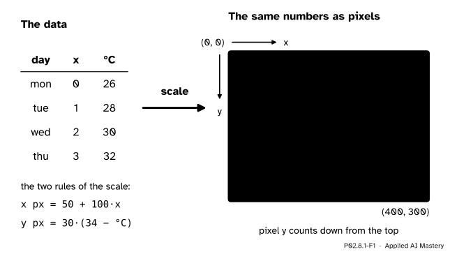
A picture on a screen is a grid of pixels. To draw the four readings, each needs a pixel position. A scale is the rule that turns a data number into a pixel position. Plotting is mostly that: two scales, one across and one up, applied to every point.

P02.8.1-F1

A plot is a scale. Each reading is turned into a pixel position in a 400 by 300 box, and the positions are joined. Note the corner: pixel \({(0, 0)}\) is at the top left, and pixel \(y\) counts down.

The scale has two choices in it. The first is the limits: which data values sit at the edges of the box. The second is the size of the box in pixels. Once both are fixed, every position follows by arithmetic, and that arithmetic is the whole of this lesson’s first half.

Build it up

Step 1. The box. Picture files count pixels from the top-left corner: \(x\) grows to the right and \(y\) grows downward. That is the convention of SVG, of PNG and of screens in general. Our box is 400 pixels wide and 300 high.

Step 2. The limits. We choose to show \(x\) from \(-0.5\) to \(3.5\), so that the four days (at positions 0, 1, 2, 3) sit away from the edges, and temperatures from 24 to 34 °C.

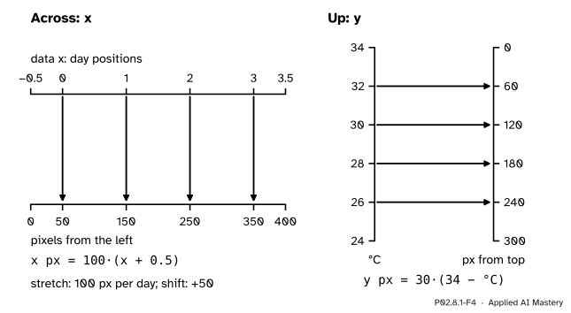
Step 3. Across. The \(x\) range is 4 days wide and the box is 400 pixels wide, so one day is 100 pixels. Position 0 is half a day from the left edge: 50 pixels. In general, a day at position \(x\) lands at \(50 + 100x\) pixels.

Step 4. Up, and the flip. The temperature range is 10 °C and the box is 300 pixels high, so 1 °C is 30 pixels. But the top of the box shows the highest value, 34 °C, and pixel \(y\) counts down from there. So we measure down from 34: a temperature \(T\) lands \({30\,(34 - T)}\) pixels below the top. For 26 °C that is \({30 \times 8} = 240\).

Step 5. The picture. An SVG file draws a line through a list of points with one element, <polyline points="50,240 150,180 250,120 350,60"/>. Writing that string is plain Python: a list of number pairs joined with spaces.

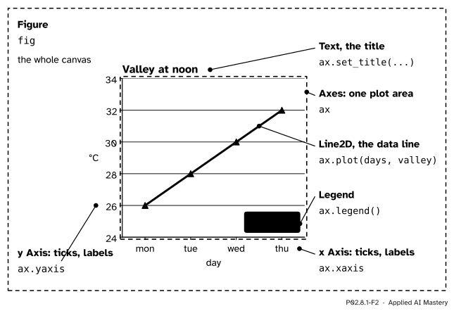
Step 6. Matplotlib does the same. fig, ax = plt.subplots() makes a Figure, the whole canvas, and one Axes, a plotting area with its own data limits. ax.plot(days, valley) adds a line. When the figure is drawn, the Axes applies a scale of the same kind as Steps 3 and 4 to every point, built from its own limits and its own box in the figure. The rule is stored on the Axes as ax.transData, and you can call it yourself.

P02.8.1-F2

The parts of a figure, named on the chart that this lesson’s code draws. Everything visible is an artist; the Axes holds the data, its two Axis objects hold the ticks.

The names are easy to mix up. An Axes (plural form, one object) is a plotting area. An Axis is one of its two number lines, ax.xaxis or ax.yaxis, with its ticks and tick labels. Everything that is drawn, from a line to a piece of text, is an artist; a line is a Line2D.

The formal statement

Definition: the scale of a plot

An Axes shows data \(x\) from \(x_{\min}\) to \(x_{\max}\) and \(y\) from \(y_{\min}\) to \(y_{\max}\) in a box \(W\) pixels wide and \(H\) pixels high. A data point \({(x, y)}\) lands at the pixel position

\[ \begin{aligned} p_x &= \frac{x - x_{\min}}{x_{\max} - x_{\min}}\, W, \\[4pt] p_y &= \frac{y_{\max} - y}{y_{\max} - y_{\min}}\, H, \end{aligned} \]

with \(p_y\) counted down from the top of the box.

Why these formulas. Take \(p_x\). The fraction \({\frac{x - x_{\min}}{x_{\max} - x_{\min}}}\) says how far along the data range \(x\) is: 0 at the left limit, 1 at the right limit, \(\tfrac12\) halfway. The pixel position is the same fraction of the width, so multiply by \(W\). For \(p_y\) the box is read from the top, where \(y_{\max}\) sits, so the fraction is measured from \(y_{\max}\) downward instead.

P02.8.1-F4

Each scale is two rulers laid side by side. Across, both rulers count the same way. Up, the data ruler counts upward and the pixel ruler counts downward, which is the flip.

Put in the lesson’s numbers: \(x_{\min} = -0.5\), \(x_{\max} = 3.5\), \(W = 400\), \(y_{\min} = 24\), \(y_{\max} = 34\), \(H = 300\). Then

\[ \begin{aligned} p_x &= \frac{x + 0.5}{4} \times 400 = 100x + 50, \\[4pt] p_y &= \frac{34 - y}{10} \times 300 = 30\,(34 - y). \end{aligned} \]

Two things follow, and both matter when you read a chart.

Equal steps stay equal. Each rule is a multiplication followed by a shift (a mathematician calls this an affine map), so a rise of 2 °C is always 60 pixels, wherever it happens. That is why the slope of a line on a chart means something.
The limits decide the look. Halve the range to 5 °C and every rise becomes twice as tall on the page. The data have not changed; only the scale has. When you do not choose limits, Matplotlib picks them from the data and pads the range by 5 per cent at each end: for 26 to 32 it shows 25.7 to 32.3.

Matplotlib’s own vocabulary, from its quick start guide: the Figure is the whole figure and keeps track of its Axes; an Axes is a region for plotting data, usually with two Axis objects that provide the ticks and tick labels; and everything visible on the figure is an Artist. In the terms of its transformations tutorial, ax.transData takes data coordinates to display coordinates, whose origin is the bottom left, so its \(y\) grows upward. To compare with a picture file, whose \(y\) grows downward, subtract from the height: \(H - y\).

Worked example

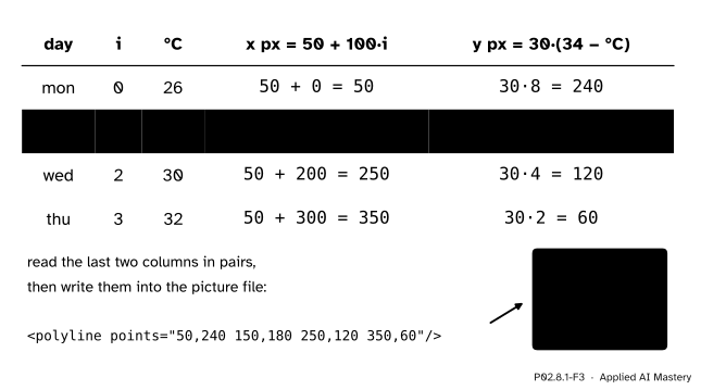
Where do the four valley readings land in the 400 by 300 box, with limits \(-0.5\) to \(3.5\) and 24 to 34?

P02.8.1-F3

The scale applied to each reading, one row per day. The pixel pairs become the points of an SVG polyline.

Take Tuesday, position 1, 28 °C.

Across: \(p_x = {100 \times 1} + 50 = 150\).
Up: \({34 - 28} = 6\) degrees below the top limit, and each degree is 30 pixels, so \(p_y = {30 \times 6} = 180\) pixels down from the top.

The other days follow the same two lines: Monday \({(50, 240)}\), Wednesday \({(250, 120)}\), Thursday \({(350, 60)}\). Read down the last column: 240, 180, 120, 60. The pixel \(y\) falls by 60 each day while the temperature rises by 2, which is the flip at work. Joined in order, the four points make a line that climbs from the lower left to the upper right, as a warming week should.

Code

The scale from scratch, in plain Python. Multiplying before dividing keeps every value exact.

import tempfile
from pathlib import Path

import matplotlib.pyplot as plt
import numpy as np

temps = np.array([[21, 19, 26], [27, 23, 28], [27, 18, 30], [29, 20, 32]])
days = ["mon", "tue", "wed", "thu"]
valley = temps[:, 2]

def scale(value, lo, hi, size):
    """How far along a ruler of `size` pixels, from lo to hi, a value lands."""
    return (value - lo) * size / (hi - lo)

xs = [scale(i, -0.5, 3.5, 400) for i in range(4)]
ys = [300 - scale(v, 24, 34, 300) for v in valley.tolist()]   # count down from the top
points = " ".join(f"{x:g},{y:g}" for x, y in zip(xs, ys))
print(xs)
print(ys)
print(points)

[50.0, 150.0, 250.0, 350.0]
[240.0, 180.0, 120.0, 60.0]
50,240 150,180 250,120 350,60

Write the picture file. Any browser opens it and draws the line.

folder = Path(tempfile.mkdtemp())
svg = ('<svg xmlns="http://www.w3.org/2000/svg" width="400" height="300">'
       f'<polyline points="{points}" fill="none" stroke="black"/></svg>')
(folder / "valley_by_hand.svg").write_text(svg, encoding="utf-8")
print(svg)

<svg xmlns="http://www.w3.org/2000/svg" width="400" height="300"><polyline points="50,240 150,180 250,120 350,60" fill="none" stroke="black"/></svg>

Now Matplotlib. A figure of 4 by 3 inches at 100 dots per inch is 400 by 300 pixels, and subplots_adjust lets the Axes fill all of it, so that its box is our box. ax.transData then gives each point’s display position, with \(y\) counted up from the bottom.

fig, ax = plt.subplots(figsize=(4, 3), dpi=100)
fig.subplots_adjust(left=0, right=1, bottom=0, top=1)
ax.plot(days, valley)
ax.set_xlim(-0.5, 3.5)
ax.set_ylim(24, 34)
display = ax.transData.transform([(i, v) for i, v in enumerate(valley.tolist())])
print(display)
print("counted from the top:", 300 - display[:, 1])
plt.close(fig)

[[ 50.  60.]
 [150. 120.]
 [250. 180.]
 [350. 240.]]
counted from the top: [240. 180. 120.  60.]

Matplotlib agrees with the hand computation. Without set_ylim, it picks the limits itself.

fig, ax = plt.subplots()
ax.plot(days, valley)
low, high = ax.get_ylim()
print(f"{low:.1f} to {high:.1f}")
plt.close(fig)

25.7 to 32.3

The chart of Figure 2 in full, built through the Axes and saved twice. The cell closes the figure instead of showing it; the lesson’s figures are drawn in the site’s own style from the same calls.

fig, ax = plt.subplots(figsize=(4, 3))
line, = ax.plot(days, valley, marker="^", label="valley")
ax.set_title("Valley at noon")
ax.set_xlabel("day")
ax.set_ylabel("°C")
ax.set_ylim(24, 34)
ax.grid(True, axis="y")
ax.legend(loc="lower right")
fig.savefig(folder / "valley.png", dpi=150)
fig.savefig(folder / "valley.svg")
print(type(fig).__name__, type(ax).__name__, type(ax.xaxis).__name__, type(line).__name__)
print(ax.get_title(), "|", ax.get_xlabel(), "|", ax.get_ylabel())
png = (folder / "valley.png").read_bytes()
print("PNG size:", int.from_bytes(png[16:20], "big"), "by", int.from_bytes(png[20:24], "big"))
plt.close(fig)

Figure Axes XAxis Line2D
Valley at noon | day | °C
PNG size: 600 by 450

A 4 by 3 inch figure saved at 150 dots per inch is 600 by 450 pixels. Many examples online use the implicit style instead, where pyplot keeps track of a “current” Figure and Axes and functions such as plt.plot act on them. Read it once, so that you can translate it.

plt.figure(figsize=(4, 3))
plt.plot(days, valley, marker="o")
plt.title("Valley at noon")
current = plt.gca()             # "get current Axes": the one plt.title just changed
print(current.get_title())
plt.close("all")

Valley at noon

plt.title(...) is plt.gca().set_title(...). This course writes the explicit form, ax.set_title(...), because then the code says which Axes it changes.

Explore

P02.8-X1

Figure anatomy

Switch each part of the chart on and off: the outline shows what it is, and the read-out names the object it belongs to and the line of code that makes it. Then move the y limits and watch the same four numbers look steep, flat or cut off.

The parts of a Matplotlib figure named on a chart of the valley temperatures: the Figure, the Axes, the title, the line, the legend, and the x and y Axis with their ticks, each with the code that makes it.

Pitfalls

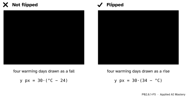
P02.8.1-F5

Wrong beside right. Measured up from the bottom but written into a file that counts down from the top, a rise turns into a fall.

“Pixel y grows upward, like a graph.”

In a picture file and on a screen, \(y\) grows downward from the top-left corner. Measure the temperature up from the bottom and write that number as the pixel \(y\), and the line is drawn upside down. Measure down from the top limit, as the formal statement does, or subtract from the height. Matplotlib’s display coordinates point up, so its numbers need the same \(H - y\) before they match a picture file.

“plt.title labels the plot I am looking at.”

It labels the current Axes, which is whichever was made or touched last. With two figures open, or several Axes in one, the title can land on the wrong one without any error. Keep the ax that plt.subplots() returns and call its methods: ax.set_title, ax.set_xlabel, ax.set_ylim.

“Matplotlib’s limits show the data as they are.”

Left to itself, Matplotlib fits the limits tightly round the data, so any change fills the height: a 6 °C rise and a 0.6 °C rise look the same. A training curve whose loss falls from 0.51 to 0.50 can look like a cliff. Read the tick labels, and set the limits yourself with ax.set_ylim when the size of a change matters.

Check yourself

Recall

1. In a picture file, where is pixel \({(0, 0)}\) and which way does \(y\) grow?

Show answer

At the top-left corner; \(x\) grows to the right and \(y\) grows downward.

2. With limits 24 to 34 °C and a box 300 pixels high, how many pixels is 1 °C?

Show answer

300 / 10 = 30 pixels.

3. What is the difference between an Axes and an Axis?

Show answer

An Axes is a whole plotting area with its own data limits. An Axis is one of its number lines (ax.xaxis or ax.yaxis), with the ticks and tick labels.

4. What does ax.transData do?

Show answer

It applies the Axes’ scale: it turns data coordinates into display coordinates (pixels), with \(y\) counted up from the bottom.

5. What does plt.title("...") change, and what does this course write instead?

Show answer

The title of the current Axes, the one made or used last. The course writes ax.set_title("...") on an Axes it holds by name.

Exercises

1. ★ The y limits are changed to 20 and 40 °C, in the same 300-pixel-high box. Where do 26 °C and 32 °C land, counted down from the top?

Show solution

1 °C is now 300 / 20 = 15 pixels. 26 °C is \({40 - 26} = 14\) degrees below the top, so \({14 \times 15} = 210\) pixels down. 32 °C is 8 degrees below the top: \({8 \times 15} = 120\) pixels. The 6 °C rise now spans 90 pixels instead of 180, so the line looks half as steep.

2. ★★ Go backwards. In the lesson’s box (limits 24 to 34, 300 pixels high), a point is drawn 90 pixels down from the top. What temperature is it? Write the general rule that turns a pixel \(p_y\) back into a data value.

Show solution

Each degree is 30 pixels, so 90 pixels is 3 degrees below the top limit: \({34 - 3} = 31\) °C. Solving \(p_y = {H\,(y_{\max} - y) / (y_{\max} - y_{\min})}\) for \(y\) gives

\[ y = y_{\max} - \frac{p_y}{H}\,(y_{\max} - y_{\min}). \]

Matplotlib holds this inverse too, as ax.transData.inverted(); it is how a click on a chart is turned back into data numbers.

3. ★★★ In a real figure the Axes does not fill the canvas. Suppose its box runs from \(x = 80\) to \(576\) pixels and from \(y = 58\) to \(427\) pixels counted from the top of a 640 by 480 figure, with the lesson’s limits. Where do Monday (position 0, 26 °C) and Thursday (position 3, 32 °C) land in the figure? Write scale so that it takes the box’s start as well.

Show solution

The box is \({576 - 80} = 496\) pixels wide and \({427 - 58} = 369\) pixels high. Across, one day is \({496 / 4} = 124\) pixels, so position \(x\) lands at \(80 + {124\,(x + 0.5)}\): Monday at \({80 + 62} = 142\) and Thursday at \({80 + 434} = 514\). Up, one degree is \(36.9\) pixels, and a temperature \(T\) lands at \(58 + {36.9\,(34 - T)}\): Monday at \({58 + 295.2} = 353.2\) and Thursday at \({58 + 73.8} = 131.8\).

def scale(value, lo, hi, start, size):
    return start + (value - lo) * size / (hi - lo)

scale(0, -0.5, 3.5, 80, 496)            # 142.0
58 + 369 - scale(26, 24, 34, 0, 369)    # 353.2, counted down from the top

Summary card

A plot is a scale: limits and a box size turn data into pixels.

P02.8.1-F1

Data in, pixels out.

Across: the fraction of the way from \(x_{\min}\) to \(x_{\max}\), times the width \(W\); here \({p_x = 100x + 50}\).
Up, flipped: the fraction of the way down from \(y_{\max}\), times the height \(H\); here \({p_y = 30\,(34 - y)}\), counted from the top.
Explicit style: fig, ax = plt.subplots(), then ax.plot, ax.set_title, ax.set_xlabel, ax.set_ylim, ax.legend, fig.savefig.
Parts: Figure (canvas) holds Axes (plot areas); each Axes has two Axis objects (ticks); everything drawn is an artist, such as a Line2D.

Sources and next steps

Sources. Each was opened and checked against this lesson on 15 November 2026.

Matplotlib developers, Quick start guide, Matplotlib 3.11.2. The section Parts of a Figure defines Figure, Axes, Axis and Artist in the words used here; Coding styles names the explicit (object-oriented) and implicit (pyplot) styles and recommends the explicit one for code that is reused.
Matplotlib developers, Transformations tutorial, Matplotlib 3.11.2. Its table of coordinate systems gives ax.transData for data coordinates and puts the origin of display coordinates at the bottom left, in pixels for the Agg backend.
W3C, Scalable Vector Graphics (SVG) 2, section 8.4, The initial coordinate system: the origin is at the top left, with \(x\) to the right and \(y\) pointing down.
MDN Web Docs, <polyline>: the points attribute is a list of \(x,y\) pairs that the element joins with straight lines.

Next. P02.8.2 Scatter, bar and histogram adds three more calls on the same Axes, one for each kind of question. The training curves of ML01.5 are this lesson’s line plot with epochs across and loss up.

This lesson unlocks

P02.8.2 Scatter, bar and histogram

Your progress is saved in this browser only. No account, no tracking.