An aggregate gives one number per group; transform sends that number back to every row of the group. Build it in two passes with a dict, compute each reading’s anomaly, z-score and share of its group, see that it matches broadcasting on the wide table, and avoid the leak of group features.
P02.6.3L1 Core25 minIn review (what this means)
The maths and code on this page are checked by automated tests on every change, but an independent reader has not signed it off yet. Spot a mistake or a confusing step? Tell us.
Explain how transform differs from an aggregation: one value per input row, under the input’s index.
Compute each reading’s anomaly, within-group z-score and share of its group total, by hand and with transform.
Show that the anomalies of a group add up to zero and that the shares of a group add up to one.
Compute a group statistic used as a feature from the training rows only.
The question
Is a noon reading of 27 warm? At the coast it is 1 degree above the station’s mean of 26. At the valley it would be 2 degrees below the mean of 29. To compare readings fairly, each one needs its own station’s mean beside it: not one row per station, but the station’s number copied onto all twelve rows. That is the second thing a group-by can do.
From the last lesson
1. Why does grouping the readings by station and sky give 7 rows and not 9?
Show answer
Only 7 of the 9 possible pairs occur. Coast with cloudy and valley with rain have no rows, so they have no group.
2. What does mean_temp=('temp', 'mean') mean inside agg?
Show answer
Named aggregation: make an output column called mean_temp that holds the mean of temp for each group.
Intuition
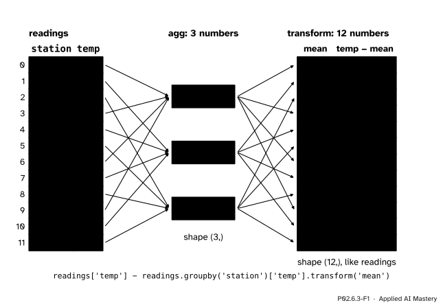
An aggregation collapses each group to one number, so the result has one row per group. A transformation computes the same number and then sends it back down to every row of the group, so the result has one row per input row, in the input’s order and under the input’s index.
P02.6.3-F1
Aggregate, then send back. The three station means fan out again to the twelve rows they came from, so each reading can be compared with its own station: its anomaly is temp minus mean.
The new column lines up with the old ones row for row, so it can be subtracted, divided or stored as a new column without any further matching. Wickham lists this use first among the places the split-apply-combine pattern appears: standardising values within groups during data preparation.
Build it up
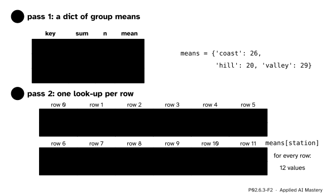
Step 1. Two passes by hand. The first pass is the group-by of lesson P02.6.1: a dictionary from each station to its mean. The second pass walks down the rows again and looks each row’s station up.
P02.6.3-F2
Transform by hand. Pass 1 builds one mean per key; pass 2 gives every row the mean of its own key.
Step 2. In pandas.transform does both passes. Given the name of a summary, it returns one value per row, indexed like the input:
The subtraction is safe because both Series carry the same twelve labels, 0 to 11, so label alignment (P02.4.4) pairs every reading with its own mean.
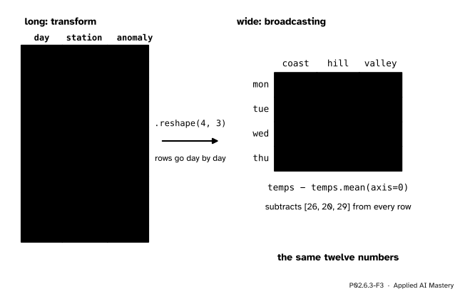
Step 3. The same numbers as broadcasting. The readings are ordered day by day and, within a day, station by station. So the twelve anomalies, read in rows of three, form the grid of the wide table minus its column means: temps - temps.mean(axis=0) from lesson P02.2.4.
P02.6.3-F3
Long or wide, the anomalies agree. A transform on the long table does what broadcasting does on the wide one; the long table also works when groups have different sizes, where no grid exists.
Step 4. Other summaries sent back. Any summary can travel back to the rows. Two are common:
a within-group z-score, (temp minus group mean) divided by the group’s standard deviation, which puts every station on the same scale;
a share of the group total, temp divided by the group’s sum, which says how much of its group a row accounts for.
pandas’ transform('std') divides by \({n - 1}\), as every pandas standard deviation does. To divide by \(n\), as NumPy does and as the coast column’s standard deviation of exactly 3 assumes, pass ddof=0: transform('std', ddof=0).
The formal statement
NoteDefinition: transformation
Let row \(i\) have key \(k_i\) and value \(x_i\), and let \(a_g\) be the aggregate of group \(g\). The transformation of the column gives row \(i\) the aggregate of its own group:
\[
t_i = a_{k_i}, \qquad i = 1, \dots, n .
\]
The result has the same length and the same index as the input. The anomaly of row \(i\) is \({d_i = x_i - m_{k_i}}\), where \(m_g\) is the mean of group \(g\). With \(s_g\) the group’s standard deviation and \(T_g\) its total, the within-group z-score is \({z_i = d_i / s_{k_i}}\) and the share is \({p_i = x_i / T_{k_i}}\).
Three facts follow, each from the definition of a group mean or total.
The anomalies of a group add up to zero. The group has \({\abs{G_g}}\) rows and their values add up to \({\abs{G_g}\, m_g}\), because that is what the mean means. So
The z-scores of a group have mean 0 and standard deviation 1, when \(s_g\) divides by the group size. Dividing every anomaly by the same \(s_g\) divides their mean by \(s_g\), and their mean is 0, so the z-scores have mean 0. Their spread is
because the mean of the squared anomalies is, by definition, \(s_g^2\). Since the z-scores have mean 0, this mean of squares is their variance, and its square root, their standard deviation, is 1.
The shares of a group add up to one. Every share in the group has the same denominator \(T_g\):
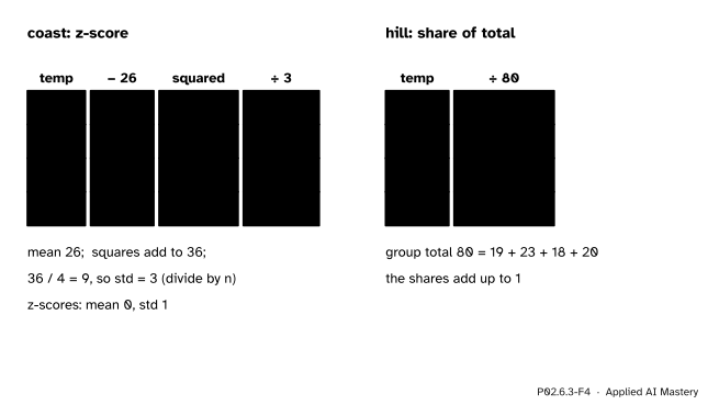
The worked example. Every column is one step of the arithmetic, applied to each row of one group.
Coast. The readings are 21, 27, 27 and 29, with mean 26. The anomalies are \({21 - 26 = -5}\), then 1, 1 and 3; they add up to \({-5 + 1 + 1 + 3 = 0}\), as the first fact promises. Squared, they are 25, 1, 1 and 9, which add up to 36. Dividing by the 4 readings gives 9, so the standard deviation is \({\sqrt{9} = 3}\). The z-scores are \({-5/3 \approx -1.67}\), \({1/3 \approx 0.33}\), 0.33 and \({3/3 = 1}\). Monday at the coast was unusually cold for the coast, by one and two thirds standard deviations.
Hill. The readings are 19, 23, 18 and 20, with total \({19 + 23 + 18 + 20 = 80}\). The shares are \({19/80 = 0.2375}\), \({23/80 = 0.2875}\), \({18/80 = 0.225}\) and \({20/80 = 0.25}\), and they add up to 1.
Code
The table, then the transform by hand in two passes:
import numpy as npimport pandas as pdtemps = np.array([[21, 19, 26], [27, 23, 28], [27, 18, 30], [29, 20, 32]])days, stations = ['mon', 'tue', 'wed', 'thu'], ['coast', 'hill', 'valley']readings = pd.DataFrame({'day': [d for d in days for s in stations],'station': stations *4,'temp': temps.ravel(),'sky': ['rain', 'rain', 'cloudy', 'clear', 'clear', 'cloudy','clear', 'cloudy', 'clear', 'clear', 'cloudy', 'clear'],})sums, counts = {}, {} # pass 1for station, temp inzip(readings['station'], readings['temp']): sums[station] = sums.get(station, 0) + temp counts[station] = counts.get(station, 0) +1means = {s: sums[s] / counts[s] for s in sums}by_hand = [temp - means[station] # pass 2for station, temp inzip(readings['station'], readings['temp'])]print(means)print(by_hand)
Finally a group mean used as a feature, the honest way. Thursday plays the test set; the station means come from Monday to Wednesday only and are then looked up for the test rows with map:
The split-apply-combine machine lives in lesson P02.6.1. Step through once with aggregate, then switch to transform and step again: the last step sends each group’s number back to every one of its rows instead of stacking one row per group.
Pitfalls
P02.6.3-F5
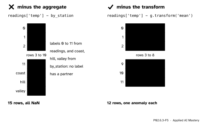
Wrong beside right. The aggregate is indexed by station, the readings by row number. Subtraction matches labels, finds no pairs and returns 15 NaN. The transform shares the readings’ labels.
“I can subtract the group means from the column directly.”
readings['temp'] - by_station lines up the labels 0 to 11 with the labels coast, hill and valley. None match, so the result has all 15 labels and every value is NaN. Use transform, or look the means up per row with readings['station'].map(by_station).
“transform(‘std’) is the standard deviation of lesson P02.2.4.”
Not quite: pandas divides by \({n - 1}\), so the coast group’s value is \({\sqrt{36/3} \approx 3.464}\), not 3. Pass ddof=0 to divide by \(n\), and say which one you used.
P02.6.3-F6
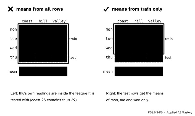
A group mean as a feature. Computed over every row, it carries the test rows’ own values into their feature; computed over the training rows only, it does not.
“A group mean is a harmless feature, so compute it on the whole table.”
If Thursday is the test set, a station mean taken over all four days contains Thursday’s own readings: the coast feature is 26 instead of 25, pulled towards the very value the model is tested on. This is leakage (lesson ML01.2.4): the score looks better than the model will be on new data. Compute the means from the training rows, then map them onto the test rows. scikit-learn’s TargetEncoder, which encodes a category by the mean target of its group pulled towards the overall mean, goes further and uses cross fitting even inside the training set.
Check yourself
Recall
1. How does the result of groupby('station')['temp'].transform('mean') differ from that of .mean()?
Show answer
.mean() gives 3 values, one per station, indexed by station. transform('mean') gives 12 values, one per reading, under the readings’ index 0 to 11.
2. What is the anomaly of Wednesday’s hill reading, 18?
Show answer
The hill mean is 20, so the anomaly is \({18 - 20 = -2}\).
3. Why do the anomalies within one group always add up to zero?
Show answer
The group’s values add up to its size times its mean, and subtracting the mean once per row takes away exactly that amount.
4. Why is readings['temp'] - readings.groupby('station')['temp'].mean() all NaN?
Show answer
Subtraction matches labels. The readings are labelled 0 to 11 and the means coast, hill, valley, so no label has a partner, and all 15 labels of the union get NaN.
5. A group mean will be a feature of a model. Which rows may it be computed from?
Show answer
From the training rows only. Computed over all rows, it carries the test rows’ values into their own features, which is leakage.
Exercises
1.★ Write down the four valley anomalies and check that they add up to zero.
Show solution
The valley readings are 26, 28, 30 and 32, with mean \({116/4 = 29}\). The anomalies are \({-3}\), \({-1}\), 1 and 3, and \({-3 - 1 + 1 + 3 = 0}\).
2.★★ Compute the hill z-scores, first dividing by \(n\) and then by \({n - 1}\), each to two decimal places.
Show solution
The hill anomalies are \({-1}\), 3, \({-2}\) and 0, whose squares add up to \({1 + 9 + 4 + 0 = 14}\).
Dividing by \({n = 4}\): the variance is \({14/4 = 3.5}\) and the standard deviation \({\sqrt{3.5} \approx 1.8708}\), so the z-scores are about \({-0.53}\), 1.60, \({-1.07}\) and 0.00. This is g.transform('std', ddof=0).
Dividing by \({n - 1 = 3}\): the variance is \({14/3}\) and the standard deviation about 2.1602, so the z-scores are about \({-0.46}\), 1.39, \({-0.93}\) and 0.00. This is pandas’ default g.transform('std').
3.★★★ Thursday is the test set. Compute Thursday’s three anomalies, once against station means taken from all four days and once against means from Monday to Wednesday only. Which pair of numbers would a model meet in use, and why do the two differ?
Show solution
From all four days the means are 26, 20 and 29, so Thursday’s readings 29, 20 and 32 have anomalies 3, 0 and 3. From Monday to Wednesday the means are \({(21 + 27 + 27)/3 = 25}\), \({(19 + 23 + 18)/3 = 20}\) and \({(26 + 28 + 30)/3 = 28}\), so the anomalies are 4, 0 and 4.
In use, a new day’s reading is compared with means built from earlier days, which is the second pair. The first pair is smaller because each mean already contains the very Thursday reading it is compared with, which pulls the mean towards that reading. Hill’s two answers agree only because its Thursday reading, 20, equals its mean over the first three days.
Summary card
Transform computes a group summary and gives it back to every row of the group.
P02.6.3-F1
One value per input row.
Transform:df.groupby(key)[col].transform('mean') has the input’s length and index.
Anomaly:x - transform('mean'); it adds up to 0 within every group.
z-score: divide the anomaly by transform('std', ddof=0) for mean 0 and std 1 per group.
Share:x / transform('sum'); the shares of a group add up to 1.
As a feature: compute group statistics on the training rows, then map them onto test rows.
Sources and next steps
Sources. Each was opened and checked against this lesson on 15 November 2026.
pandas developers, Group by: split-apply-combine, pandas 3.1.1 User Guide, section Transformation: a transformation is a GroupBy operation whose result is indexed the same as the one being grouped, and outputs of lower dimension are broadcast to match the shape of the input.
Hadley Wickham, The Split-Apply-Combine Strategy for Data Analysis, Journal of Statistical Software 40(1), 2011. Section 1 lists group-wise ranking, standardisation and normalisation during data preparation as uses of the strategy.
scikit-learn developers, Common pitfalls and recommended practices, scikit-learn 1.9.1 User Guide, Section 12.2, Data leakage: preprocessing statistics, such as the average used to normalise, must be learnt from the training data only.
scikit-learn developers, Preprocessing data, scikit-learn 1.9.1 User Guide, Section 8.3.4.2, Target Encoder: a category is encoded by the target mean of its group, shrunk towards the global target mean, and fit_transform uses cross fitting so that target information does not leak into the training representation.