One number per group is rarely enough: a mean needs its count beside it. Ask a group-by for several summaries with agg and named aggregation, group by two columns at once, flatten the two-level result with reset_index, and meet value_counts, the class balance to check before training.
P02.6.2L1 Core25 minIn review (what this means)
The maths and code on this page are checked by automated tests on every change, but an independent reader has not signed it off yet. Spot a mistake or a confusing step? Tell us.
Compute several summaries per group with agg, using a list of functions or named aggregation.
Group by two key columns and explain why the result holds only the pairs that occur.
Turn index levels back into columns with reset_index or as_index=False.
Use value_counts to check the class balance of a column before training a classifier.
The question
By sky, the mean noon temperatures are 28 for clear, 23 for cloudy and 20 for rain. But the rain mean rests on 2 readings and the clear mean on 6. A mean shown without its count invites you to trust it more than it deserves. How do you get both numbers from one group-by? And how do you ask about station and sky together?
From the last lesson
1. What does readings.groupby('station')['temp'].mean() return?
Show answer
A Series with the index coast, hill, valley (named station) and the values 26, 20 and 29.
2. In what order does readings.groupby('day')['temp'].mean() list the days, and why?
Show answer
mon, thu, tue, wed: pandas sorts the keys, and text sorts letter by letter. sort=False keeps the order of first appearance.
Intuition
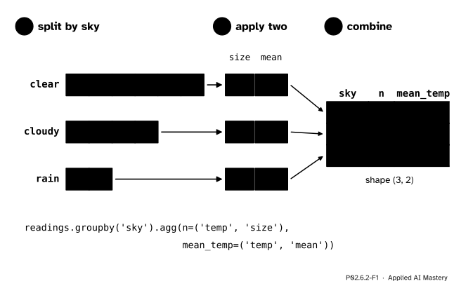
The split does not care how many summaries follow it. Once the rows sit in their piles, each pile can be asked several questions: how many rows, what mean, what maximum. Each answer becomes one column of the result, and each pile still gives one row.
P02.6.2-F1
One split, two summaries. Every pile gives one row with two numbers, so the result has one row per sky and one column per summary.
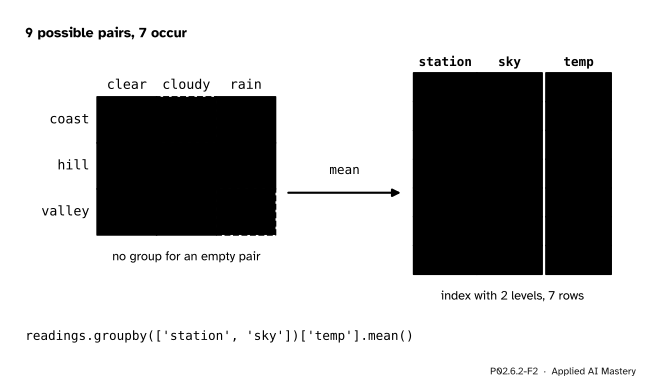
A key can also be two columns. Then a group is every row that shares both values, such as hill readings under a cloudy sky. Think of the possible pairs as a grid of 3 stations by 3 skies: the group-by fills only the cells that have rows in them.
Build it up
Step 1. A list of summaries.agg takes a list of function names and returns one column for each:
Each output names its own input column, so one call can summarise different columns: days=('day', 'nunique') adds how many different days each sky was seen on.
Step 3. Two keys. Pass a list of key columns. The result is indexed by pairs, a two-level index, and holds one row per pair that occurs.
P02.6.2-F2
Grouping by station and sky. Of the nine possible pairs, coast in cloudy weather and valley in rain never happen, so they get no group at all, not a group with the value 0.
A two-level result is read with a pair of labels: two.loc[('hill', 'cloudy')] is 19, and two.loc['hill'] gives all of hill’s skies.
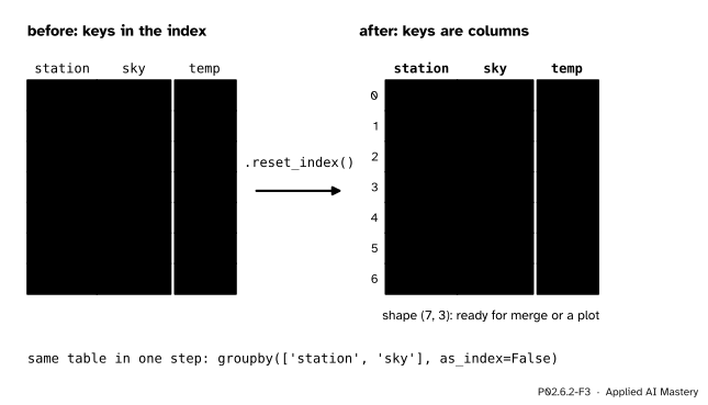
Step 4. Back to plain columns. An index with levels is compact for reading but awkward for the next step, such as a merge (P02.5.4) or a seaborn plot (P02.8.4), which want ordinary columns. reset_index() moves the levels into columns and numbers the rows from 0; as_index=False in the groupby call gives the same table directly.
P02.6.2-F3
reset_index turns the two index levels into ordinary columns and gives the rows fresh numbers.
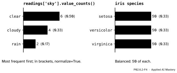
Step 5. The everyday special case. Counting the rows of each value of one column is so common that it has its own method. readings['sky'].value_counts() gives clear 6, cloudy 4, rain 2, the most frequent first, and normalize=True turns the counts into shares.
P02.6.2-F4
value_counts is groupby(column).size(), sorted with the largest group first. On a label column it is the class balance: iris has 50 flowers of each species.
Check the class balance before you train a classifier. If 990 of 1,000 rows are one class, a model that always answers that class is 99 percent accurate and useless, the trap of lesson ML01.7.1.
The formal statement
NoteDefinition: several summaries and several keys
Several summaries.agg applies each function it is given to every group. With a list, the output columns take the functions’ names. With named aggregation, name=(column, function), each output column has the given name and summarises the given input column.
Several keys. With a list of key columns, the group of a tuple of values \({(g, h)}\) is the set of rows whose first key is \(g\) and whose second key is \(h\). The result has one row for every tuple that occurs, indexed by a MultiIndex, an index with one level per key.
Counting values.s.value_counts() equals s.groupby(s).size() sorted from the largest count to the smallest. With normalize=True each count \(n_g\) is divided by the number of rows \(n\).
How many groups can there be? With \(a\) distinct values in the first key and \(b\) in the second, there are \({a \times b}\) possible pairs, so at most \({a \times b}\) groups. The readings have \({3 \times 3 = 9}\) possible pairs and 7 groups. There can also be no more groups than rows, since every group holds at least one row: 7 is at most 12.
The shares add up to one. The groups split the rows (lesson P02.6.1), so their sizes add up to \(n\). Dividing every size by \(n\) therefore gives shares that add up to 1:
By sky, \({6/12 + 4/12 + 2/12 = 1}\). The same holds for two keys: the seven pair sizes 3, 1, 1, 2, 1, 2, 2 add up to 12.
Worked example
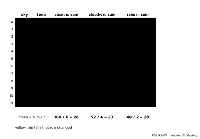
Size and mean by sky, as a hand tally. Keep a running pair (size, sum) for each sky. Walk down the 12 readings; each row adds 1 to the size and its temperature to the sum of its own sky. At the end, divide.
P02.6.2-F5
The hand tally. Each row changes one tally only, the one of its own sky (yellow). The last row of tallies holds every group’s size and sum.
Rows 0 and 1 are rain: the rain tally becomes (1, 21), then (2, 40).
Rows 2 to 11 alternate between clear and cloudy. Clear collects 27, 23, 27, 30, 29 and 32, so its tally grows (1, 27), (2, 50), (3, 77), (4, 107), (5, 136), (6, 168). Cloudy collects 26, 28, 18 and 20: (1, 26), (2, 54), (3, 72), (4, 92).
Divide. Clear \({168/6 = 28}\), cloudy \({92/4 = 23}\), rain \({40/2 = 20}\). The named aggregation of the anchor figure gives the same table: n is 6, 4, 2 and mean_temp is 28, 23, 20.
Check. The sizes add up to \({6 + 4 + 2 = 12}\) rows and the sums to \({168 + 92 + 40 = 300}\), the total of all 12 readings.
Code
The table of lesson P02.6.1, then the hand tally of the worked example:
import numpy as npimport pandas as pdtemps = np.array([[21, 19, 26], [27, 23, 28], [27, 18, 30], [29, 20, 32]])days, stations = ['mon', 'tue', 'wed', 'thu'], ['coast', 'hill', 'valley']readings = pd.DataFrame({'day': [d for d in days for s in stations],'station': stations *4,'temp': temps.ravel(),'sky': ['rain', 'rain', 'cloudy', 'clear', 'clear', 'cloudy','clear', 'cloudy', 'clear', 'clear', 'cloudy', 'clear'],})tally = {}for sky, temp inzip(readings['sky'], readings['temp']): n, total = tally.get(sky, (0, 0)) tally[sky] = (n +1, total + temp)print(tally)print({sky: total / n for sky, (n, total) in tally.items()})
The split-apply-combine machine lives in lesson P02.6.1. Choose the key sky and step through with the summary count, then with mean: the counts 6, 4 and 2 are the sizes that the means rest on.
Pitfalls
P02.6.2-F6
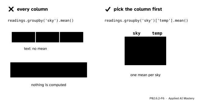
Wrong beside right. Without a column, the mean is applied to every column, including the text columns day and station, and pandas stops. Select the column to summarise first.
“groupby(‘sky’).mean() averages the temperatures.”
It tries to average every column that is not a key. day and station hold text, which has no mean, so pandas 3 raises a TypeError. Select the column first, groupby('sky')['temp'], or name each output with named aggregation.
“Grouping by station and sky gives all nine pairs.”
It gives the seven pairs that occur. Valley in rain has no row, so it has no group, and ('valley', 'rain') in two.index is False. A missing pair is not a zero; lesson P02.6.4 shows how the grid layout makes the gaps visible.
“value_counts lists the values in alphabetical order.”
It lists them by count, largest first, which happens to be alphabetical for the sky column. Use .sort_index() when you want the labels in order.
Check yourself
Recall
1. What do the columns of readings.groupby('sky')['temp'].agg(['size', 'mean']) hold?
Show answer
size holds the number of rows of each sky (6, 4, 2) and mean their mean temperature (28, 23, 20).
2. What does mean_temp=('temp', 'mean') mean inside agg?
Show answer
Named aggregation: make an output column called mean_temp holding the mean of the input column temp for each group.
3. Why does grouping the readings by station and sky give 7 rows and not 9?
Show answer
Only 7 of the 9 possible pairs occur; coast with cloudy and valley with rain have no rows, so they have no group.
4. What do reset_index() and as_index=False do to a group-by result?
Show answer
They turn the key levels of the index into ordinary columns and number the rows from 0.
5. What does readings['sky'].value_counts(normalize=True) give?
Show answer
The share of rows for each sky, largest first: clear 0.5, cloudy about 0.33, rain about 0.17. The shares add up to 1.
Exercises
1.★ Find the lowest and the highest temperature under each sky with one agg call.
Show solution
readings.groupby('sky')['temp'].agg(['min', 'max']) gives clear 23 and 32, cloudy 18 and 28, rain 19 and 21. By hand, the clear pile is 27, 23, 27, 30, 29, 32, the cloudy pile 26, 28, 18, 20 and the rain pile 21, 19.
2.★★ Build a table by station with named aggregation: the number of readings n, the mean mean_temp and the highest hottest. Then use two keys to list the (station, sky) pairs with at least two readings.
gives coast 4, 26, 29; hill 4, 20, 23; valley 4, 29, 32. For the pairs, sizes = readings.groupby(['station', 'sky']).size() and sizes[sizes >= 2] keep four pairs: (coast, clear) with 3, (hill, cloudy) with 2, (valley, clear) with 2 and (valley, cloudy) with 2.
3.★★★ Count the (station, sky) pairs by hand with a dictionary whose keys are tuples, check that the counts add up to 12, and explain why a table with \(n\) rows and two keys with \(a\) and \(b\) distinct values has at most the smaller of \({a \times b}\) and \(n\) groups.
pairs holds 7 keys: (coast, rain) 1, (hill, rain) 1, (valley, cloudy) 2, (coast, clear) 3, (hill, clear) 1, (hill, cloudy) 2, (valley, clear) 2, in the order they are first met. The counts add up to 12 because every row adds 1 to exactly one count. A group is one pair of values, and there are only \({a \times b}\) pairs, so there are at most \({a \times b}\) groups. Every group holds at least one row and no row is in two groups, so there are also at most \(n\) groups. Both limits hold at once, so the number of groups is at most the smaller one: here the smaller of 9 and 12.
Summary card
Ask each group several questions; group by several columns at once.
P02.6.2-F1
One row per group, one column per summary.
Several summaries:.agg(['size', 'mean']), or named: .agg(n=('temp', 'size')).
Several keys:groupby(['station', 'sky']) gives one row per pair that occurs, under a MultiIndex.
Flatten:.reset_index(), or as_index=False.
Count values:s.value_counts(), largest first; with normalize=True the shares add up to 1.
Sources and next steps
Sources. Each was opened and checked against this lesson on 15 November 2026.
pandas developers, Group by: split-apply-combine, pandas 3.1.1 User Guide. Aggregation computes a summary statistic for each group; named aggregation takes keywords that are the output column names and values that are tuples of (column, aggregation), with pd.NamedAgg as a named tuple; as_index=False puts the keys in columns instead of the index.
pandas developers, Series.value_counts, pandas 3.1.1 API reference: counts of unique values in descending order, the most frequent first; normalize=True gives relative frequencies.
pandas developers, DataFrame.groupby, pandas 3.1.1 API reference: as_index=True returns the group labels as the index, and as_index=False gives “SQL-style” grouped output.