\( \newcommand{\vect}[1]{\boldsymbol{\mathbf{#1}}} \newcommand{\mat}[1]{\boldsymbol{\mathbf{#1}}} \newcommand{\R}{\mathbb{R}} \newcommand{\E}{\mathbb{E}} \newcommand{\Prob}{\mathbb{P}} \newcommand{\T}{^{\top}} \newcommand{\norm}[1]{\lVert #1 \rVert} \newcommand{\abs}[1]{\lvert #1 \rvert} \newcommand{\ihat}{\mkern1mu\hat{\boldsymbol{\imath}}\mkern2mu} \newcommand{\jhat}{\mkern1mu\hat{\boldsymbol{\jmath}}\mkern2mu} \newcommand{\pd}[2]{\frac{\partial #1}{\partial #2}} \newcommand{\argmax}{\operatorname*{arg\,max}} \newcommand{\argmin}{\operatorname*{arg\,min}} \newcommand{\cdata}[1]{\class{c-data}{#1}} \newcommand{\cmodel}[1]{\class{c-model}{#1}} \newcommand{\ctruth}[1]{\class{c-truth}{#1}} \newcommand{\cgrad}[1]{\class{c-grad}{#1}} \newcommand{\closs}[1]{\class{c-loss}{#1}} \newcommand{\cparam}[1]{\class{c-param}{#1}} \newcommand{\csecond}[1]{\class{c-second}{#1}} \renewcommand{\,}{\mkern3mu} \)

Split, apply, combine

A group-by is three steps: split the rows into one pile per key, apply a summary to each pile, combine the answers into one table. Do all three by hand on the weather readings with a dict of lists, then in one line of pandas, and learn why the keys come back sorted.

P02.6.1L1 Core25 min

In review

The maths and code on this page are checked by automated tests on every change, but an independent reader has not signed it off yet. Spot a mistake or a confusing step? Tell us.

Before this lesson: P02.5 Cleaning, reshaping and joining P02.4 DataFrames and Series

What you will be able to do

Describe a group-by as split, apply and combine, and carry out all three by hand with a dict of lists.
Compute a summary per group with groupby and read the result as a Series indexed by the sorted keys.
Show that the overall mean is the mean of the group means weighted by group size, and check it on the readings.
Tell size from count when a group holds a missing value.

The question

The long table readings holds 12 noon temperatures: three stations on four days. What is the mean temperature at each station? You could filter the table three times and average each piece. Now imagine 400 stations, or a million customers, or the 50 flowers of each iris species. There must be one operation that answers “a number per group” in a single step. There is, and it has three parts.

Intuition

The readings are the course’s small world: three weather stations, coast, hill and valley, read at noon from Monday 3 to Thursday 6 March 2025. Every number is invented for teaching. In the long form of lesson P02.5.3 each reading is one row, with columns day, station, temp and sky.

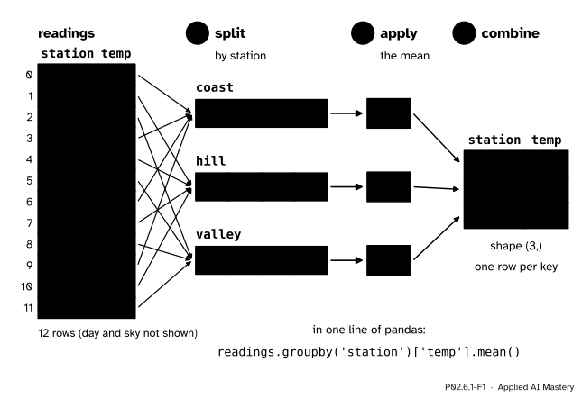
To get one mean per station, do what you would do with paper slips. Split the slips into one pile per station. Apply the mean to each pile, so that each pile collapses to one number. Combine the three numbers into a small table, one row per station.

P02.6.1-F1

Split, apply, combine. The station column is the key: it decides which pile each row joins. Twelve rows go in; one row per key comes out.

The column that decides the piles is the key, drawn in orange because it steers the operation. The rows that share a key value form a group. The whole three-step operation is called a group-by, after the SQL words GROUP BY. Hadley Wickham named the three steps in 2011 and pointed out that the same pattern hides inside spreadsheet pivot tables, SQL and map-reduce.

Machine learning meets it constantly. The mean of the target in each category is the simplest model there is: predict tomorrow’s coast reading with the coast mean. It is also how features are built (“mean spend per customer”) and how results are reported (“accuracy per class”).

Build it up

Step 1. Choose the key. The key is a column whose values name the groups. station has three distinct values, so there will be three groups of four rows each.

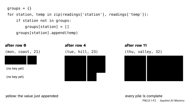
Step 2. Split by hand. One pass over the rows fills a dictionary from key to a list of values. The first time a key is met it gets an empty list; every row appends its temperature to the list of its key.

P02.6.1-F2

Splitting by hand. Each row appends its value to the list of its key; the yellow slot is the value the last row added. After all 12 rows the three piles of the anchor figure are complete.

Step 3. Apply. Each list collapses to one number. For coast, \({(21 + 27 + 27 + 29)/4 = 104/4 = 26}\); for hill, \({80/4 = 20}\); for valley, \({116/4 = 29}\).

Step 4. Combine. The three numbers become one table, indexed by the key: a Series with the index coast, hill, valley and the values 26, 20, 29. Building pd.Series(means) from the dictionary does exactly that.

Step 5. The same in one line. pandas does all three steps in one expression:

readings.groupby('station')['temp'].mean()

Read it left to right. groupby('station') makes the split and keeps it as a plan: which row positions belong to which key. ['temp'] picks the column to summarise. .mean() applies the mean to each group and combines the answers into a Series whose index is the key.

The formal statement

Definition: group-by

Take a table of \(n\) rows with a key column \(k\) and a value column \(x\). The group of a key value \(g\) is the set of row positions \(G_g\) whose key equals \(g\). Every row has exactly one key value, so the groups split the rows into separate piles that together hold every row.

An aggregation \(f\) turns the values of one group into one number, \({a_g = f(\{x_i : i \in G_g\})}\). The result of the group-by is one \(a_g\) per key, indexed by the keys, which pandas sorts unless told sort=False.

The size of a group is the number of its rows, \({\abs{G_g}}\). Its count is the number of its values that are not missing. They differ only when a group holds a missing value.

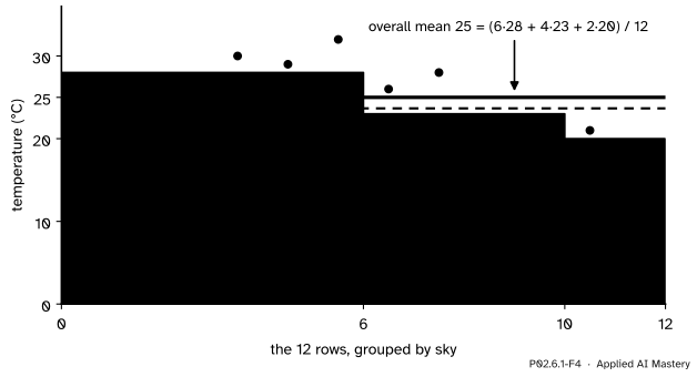
Because the groups split the rows, their sizes add up to \(n\): \({4 + 4 + 4 = 12}\) by station, and \({6 + 4 + 2 = 12}\) by sky, where clear, cloudy and rain cover 6, 4 and 2 readings.

How the group means build the overall mean. Write \(m_g\) for the mean of group \(g\), so that the sum of the group’s values is \({\abs{G_g}\, m_g}\). The overall mean \(\bar{x}\) adds every value once. Since every row sits in exactly one group, the sum can be taken group by group:

\[ \begin{aligned} \bar{x} &= \frac{1}{n} \sum_{i=1}^{n} x_i \\ &= \frac{1}{n} \sum_{g} \sum_{i \in G_g} x_i \\ &= \frac{1}{n} \sum_{g} \abs{G_g}\, m_g \\ &= \sum_{g} \frac{\abs{G_g}}{n}\, m_g . \end{aligned} \]

The second line regroups the sum by pile; the third replaces each pile’s sum by size times mean. So the overall mean is the mean of the group means weighted by group size. By sky:

\[ \begin{aligned} \bar{x} &= \frac{6 \cdot 28 + 4 \cdot 23 + 2 \cdot 20}{12} \\ &= \frac{168 + 92 + 40}{12} = \frac{300}{12} = 25 . \end{aligned} \]

P02.6.1-F4

Each group is a block as wide as its size and as tall as its mean. The overall mean is the height of one block of the same total area: 25. The plain average of the three heights, 23.67, gives the small rain group as much say as the large clear group.

When every group has the same size, every weight is \({1/3}\) and the plain average of the means is right: by station, \({(26 + 20 + 29)/3 = 25}\). By sky it is not, since \({(28 + 23 + 20)/3}\) is about 23.67. Lesson P02.6.4 meets this again in the margins of a pivot table.

Worked example

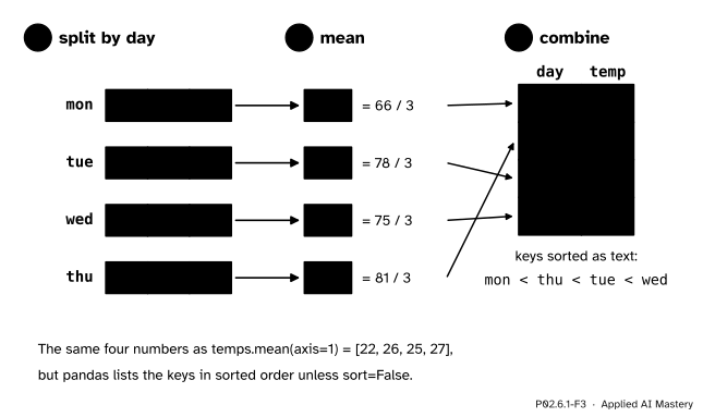
The mean temperature of each day, by hand. Split by day, apply the mean, combine.

P02.6.1-F3

The worked example. The arithmetic is the row means of P02.2.2; only the order of the result is new.

Split. Each day has three readings, one per station: Monday 21, 19, 26; Tuesday 27, 23, 28; Wednesday 27, 18, 30; Thursday 29, 20, 32.

Apply. Monday: \({21 + 19 + 26 = 66}\), and \({66/3 = 22}\). Tuesday: \({27 + 23 + 28 = 78}\), mean 26. Wednesday: \({27 + 18 + 30 = 75}\), mean 25. Thursday: \({29 + 20 + 32 = 81}\), mean 27.

Combine. pandas lists the keys in sorted order, and the days are text, so they are compared letter by letter. 'mon' comes first, because m comes before t and w. 'thu' and 'tue' share their first letter, and h comes before u, so 'thu' comes before 'tue'. 'wed' is last. The result reads mon 22, thu 27, tue 26, wed 25.

Check. Every day has three readings, so the plain average of the day means is the overall mean: \({(22 + 26 + 25 + 27)/4 = 100/4 = 25}\), as the formula above promises for equal sizes.

Code

First the table. The sky column follows the course’s outline: rain, rain, cloudy on Monday, and so on.

import numpy as np
import pandas as pd

temps = np.array([[21, 19, 26], [27, 23, 28], [27, 18, 30], [29, 20, 32]])
days = ['mon', 'tue', 'wed', 'thu']
stations = ['coast', 'hill', 'valley']
readings = pd.DataFrame({
    'day': [d for d in days for s in stations],
    'station': stations * 4,
    'temp': temps.ravel(),
    'sky': ['rain', 'rain', 'cloudy', 'clear', 'clear', 'cloudy',
            'clear', 'cloudy', 'clear', 'clear', 'cloudy', 'clear'],
})
print(readings.shape)
print(readings.head(4))

(12, 4)
   day station  temp     sky
0  mon   coast    21    rain
1  mon    hill    19    rain
2  mon  valley    26  cloudy
3  tue   coast    27   clear

Split, apply and combine from scratch, for any key column:

def group_mean(keys, values):
    groups = {}                                   # split
    for key, value in zip(keys, values):
        if key not in groups:
            groups[key] = []
        groups[key].append(value)
    means = {}                                    # apply
    for key, pile in groups.items():
        means[key] = sum(pile) / len(pile)
    return pd.Series(means)                       # combine

print(group_mean(readings['station'], readings['temp']).to_dict())
print(group_mean(readings['day'], readings['temp']).to_dict())

{'coast': 26.0, 'hill': 20.0, 'valley': 29.0}
{'mon': 22.0, 'tue': 26.0, 'wed': 25.0, 'thu': 27.0}

The hand-made version keeps the keys in the order it met them. pandas sorts them:

by_station = readings.groupby('station')['temp'].mean()
by_day = readings.groupby('day')['temp'].mean()
in_order = readings.groupby('day', sort=False)['temp'].mean()
print(by_station)
print(list(by_day.index), by_day.tolist())
print(list(in_order.index), in_order.tolist())

station
coast     26.0
hill      20.0
valley    29.0
Name: temp, dtype: float64
['mon', 'thu', 'tue', 'wed'] [22.0, 27.0, 26.0, 25.0]
['mon', 'tue', 'wed', 'thu'] [22.0, 26.0, 25.0, 27.0]

The GroupBy object itself is the split, kept as row positions until a summary is applied:

g = readings.groupby('station')
print(g.ngroups, {k: list(v) for k, v in g.groups.items()})
for key, part in g:
    print(key, part['temp'].tolist())

3 {'coast': [0, 3, 6, 9], 'hill': [1, 4, 7, 10], 'valley': [2, 5, 8, 11]}
coast [21, 27, 27, 29]
hill [19, 23, 18, 20]
valley [26, 28, 30, 32]

Finally size and count. A copy of the table loses Tuesday’s hill reading (row 4); the column becomes float first, because only floats can hold NaN.

gaps = readings.copy()
gaps['temp'] = gaps['temp'].astype(float)
gaps.loc[4, 'temp'] = np.nan
per = gaps.groupby('station')['temp']
print(per.size().tolist(), per.count().tolist(), per.mean().tolist())

[4, 4, 4] [4, 3, 4] [26.0, 19.0, 29.0]

size still counts four hill rows; count counts three values; and the mean skips the gap, giving \({(19 + 18 + 20)/3 = 19}\).

Explore

P02.6-X1

Split-apply-combine machine

Choose a key and a summary, then press Step to watch the rows split into piles, each pile collapse to one number and the numbers combine. Try the key day and see the keys come out sorted; then switch to transform, which lesson P02.6.3 explains.

The anchor figure: the 12 readings slide into three piles by station, each pile collapses to its mean, 26, 20 and 29, and the means stack into a result table indexed by station.

Pitfalls

P02.6.1-F5

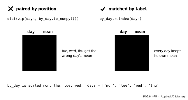
Wrong beside right. The result is sorted mon, thu, tue, wed. Pairing its values with the days in calendar order shifts three of them; matching by label keeps each mean with its day.

“The result lists the groups in the order of the rows.”

It lists them sorted by key, so the days come back as mon, thu, tue, wed. Look values up by label (by_day['tue']), reorder with reindex, or pass sort=False to keep the order of first appearance. Never pair the values with another list by position.

“groupby(‘station’) has computed the groups’ numbers.”

It has only made the plan of the split. Printing it shows a GroupBy object, not numbers. Nothing is summarised until you apply something: .mean(), .size(), .max() and the rest.

“size and count are the same thing.”

size counts rows and count counts values that are not missing. With Tuesday’s hill reading missing, hill has size 4 and count 3. When the number of usable values matters, as it does for a mean, report count.

“Labels that look alike fall into one group.”

A key is matched exactly, so 'coast', 'Coast' and 'coast ' make three groups. Clean text keys before grouping; lesson P02.7.3 shows how.

Check yourself

Recall

1. Name the three steps of a group-by and say what each does.

Show answer

Split the rows into one group per key value; apply a summary to each group, so that it becomes one number; combine the numbers into one table indexed by the key.

2. What does readings.groupby('station')['temp'].mean() return?

Show answer

A Series named temp with the index coast, hill, valley (named station) and the values 26, 20 and 29.

3. In what order does readings.groupby('day')['temp'].mean() list the days, and why?

Show answer

mon, thu, tue, wed. pandas sorts the keys, and text sorts letter by letter. sort=False keeps mon, tue, wed, thu.

4. A group has four rows and one of its values is missing. What are its size and its count?

Show answer

Size 4, count 3. Size counts rows; count skips missing values.

5. By sky the group means are 28, 23 and 20 for groups of 6, 4 and 2 rows. Why is the overall mean not their plain average?

Show answer

Each group mean must be weighted by its group’s share of the rows: \({(6 \cdot 28 + 4 \cdot 23 + 2 \cdot 20)/12} = 25\), while the plain average, about 23.67, gives the two rain rows as much weight as the six clear rows.

Exercises

1. ★ Find the highest temperature at each station, first from the piles of the anchor figure, then with pandas.

Show solution

The piles are coast 21, 27, 27, 29; hill 19, 23, 18, 20; valley 26, 28, 30, 32. Their maxima are 29, 23 and 32. In pandas, readings.groupby('station')['temp'].max() gives the same three numbers, indexed coast, hill, valley.

2. ★★ Split the readings by sky by hand and find each group’s mean. Then use the weighted formula to check the overall mean.

Show solution

Clear: Tuesday coast and hill, Wednesday coast and valley, Thursday coast and valley, that is 27, 23, 27, 30, 29, 32, sum 168, mean \({168/6 = 28}\). Cloudy: 26, 28, 18, 20, sum 92, mean 23. Rain: 21 and 19, sum 40, mean 20. The weighted formula gives \({(6 \cdot 28 + 4 \cdot 23 + 2 \cdot 20)/12} = {300/12} = 25\), the overall mean of all 12 readings.

3. ★★★ Generalise group_mean to group_agg(keys, values, f), which applies any function f to each pile. Use it to compute the range (largest minus smallest) of each station, and check the result with readings.groupby('station')['temp'].agg(lambda s: s.max() - s.min()).

Show solution

Replace the apply step with f:

def group_agg(keys, values, f):
    groups = {}
    for key, value in zip(keys, values):
        groups.setdefault(key, []).append(value)
    return pd.Series({key: f(pile) for key, pile in groups.items()})

group_agg(readings['station'], readings['temp'], lambda p: max(p) - min(p))

The ranges are coast \({29 - 21 = 8}\), hill \({23 - 18 = 5}\) and valley \({32 - 26 = 6}\). The pandas version agrees. setdefault(key, []) returns the key’s list, creating an empty one first if the key is new, so it does the job of the if in the lesson’s version.

Summary card

Split the rows by key, apply a summary to each group, combine one row per key.

The anchor figure again: 12 readings slide into three piles by station, each pile collapses to its mean, 26, 20 and 29, and the means stack into a result indexed by station. — P02.6.1-F1
Twelve rows in, one row per key out.

One line: df.groupby(key)[column].mean(); any summary can replace mean.
Keys come back sorted (mon, thu, tue, wed) unless sort=False.
size counts rows, count counts values that are not missing.
Overall mean is \({\sum_g (\abs{G_g}/n)\, m_g}\), the size-weighted mean of the group means.

Sources and next steps

Sources. Each was opened and checked against this lesson on 15 November 2026.

Hadley Wickham, The Split-Apply-Combine Strategy for Data Analysis, Journal of Statistical Software 40(1), 2011. The abstract and Section 1 define the strategy (break a problem into pieces, operate on each piece independently, put the pieces back together) and relate it to map-reduce, Excel’s pivot tables and the SQL group by operator.
pandas developers, Group by: split-apply-combine, pandas 3.1.1 User Guide: the three steps; group keys are sorted by default and sort=False keeps their order of appearance; count computes the number of non-NA values and size the number of values in each group.
pandas developers, DataFrame.groupby, pandas 3.1.1 API reference: sort defaults to True, and groupby keeps the order of rows within each group.

Next. P02.6.2 Several summaries, several keys asks for more than one number per group, and groups by two columns at once.

This lesson unlocks

P02.6.2 Several summaries, several keys

Your progress is saved in this browser only. No account, no tracking.