Nearly collinear features make the condition number of a design matrix explode, so that one nudged data point swings the fitted coefficients. Measure it on Hilbert and polynomial matrices, count the digits it costs, and test three remedies: standardising, QR and ridge.
M03.8.3L2 Intermediate25 minIn review (what this means)
The maths and code on this page are checked by automated tests on every change, but an independent reader has not signed it off yet. Spot a mistake or a confusing step? Tell us.
Explain why nearly collinear columns give a small singular value and a large condition number.
Measure how fast kappa grows for Hilbert and polynomial design matrices, and apply the rule that about log10 kappa digits are lost.
Derive kappa(A-transpose A + alpha I) = (sigma_1^2 + alpha) / (sigma_n^2 + alpha) and use it to choose a ridge strength.
Judge which remedy (standardising, QR or ridge) treats which cause of ill-conditioning.
The question
Two sensors measure the same quantity and agree to within 0.02. A regression on both fits the targets exactly with weights \({(1, 1)}\). Raise one of the four targets by 0.1, and the weights become \({(-0.25, 2.25)}\): the first sensor now counts against the answer. Nothing about the data changed in any way that matters. What went wrong, and how do practitioners protect a fit from it?
From the last lesson
1. State the bound that the condition number gives for \({\mat{A}\vect{x} = \vect{b}}\).
2. What is \({\kappa(\mat{A}\T\mat{A})}\) in terms of \({\kappa(\mat{A})}\)?
Show answer
\({\kappa(\mat{A})^2}\), because \(\mat{A}\T\mat{A} = \mat{V}\mat{\Sigma}^2\mat{V}\T\) has singular values \(\sigma_i^2\).
Intuition
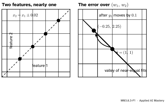
Put the two sensor readings side by side as the columns of a design matrix \(\mat{A}\). The first column is \({\vect{x}_1 = (1, 2, 3, 4)}\) and the second is \({\vect{x}_2 = \vect{x}_1 + (0.02, -0.02, -0.02, 0.02)}\). The targets are \({\vect{y} = \vect{x}_1 + \vect{x}_2}\).
M03.8.3-F1
Left: each row of the data as a point; the two features almost coincide. Right: the squared error over all weight pairs is a valley 274 times longer than it is wide. Nudging one target slides the best fit far along the floor.
Because \(\vect{x}_1\) and \(\vect{x}_2\) are nearly equal, the model can trade weight between them almost for free: \({(1, 1)}\), \({(0, 2)}\) and \({(2, 0)}\) all predict nearly the same values. The squared error is a long, narrow valley along the line \({w_1 + w_2 = 2}\). The data pins the fit down across the valley, but hardly at all along it, so a tiny change in the data moves the bottom a long way. That valley is ill-conditioning, seen from the side of the weights.
Build it up
Step 1. A near-repeat makes a small singular value. The smallest stretch \(\sigma_n\) is at most the stretch of any particular vector. Try \({\vect{z} = (1, -1)}\), which subtracts the columns:
Here the bound is almost exact: \({\sigma_2 \approx 0.0283}\). With \({\sigma_1 \approx 7.75}\), the condition number is \({\kappa(\mat{A}) \approx 274}\), and \({\kappa(\mat{A}\T\mat{A}) \approx 75\,000}\).
Step 2. The weak direction is the valley. The right singular vector for \(\sigma_2\) is close to \({(1, -1)/\sqrt2}\). Along it, a large change of weights makes a tiny change of predictions, which is exactly why the data cannot fix it.
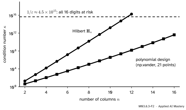
Step 3. It gets worse with size. Real designs have many columns, and some families are famous for near-dependence. The Hilbert matrix\(\mat{H}_n\) has entries \({1/(i + j - 1)}\). A polynomial design has columns \(1, x, x^2, \dots\) evaluated at data points; np.vander builds it. Both have columns that look more and more alike as \(n\) grows.
M03.8.3-F2
Condition numbers of Hilbert matrices and of polynomial designs on 21 equally spaced points in \([0, 1]\), on a log scale. Each extra column multiplies \(\kappa\) by a roughly constant factor.
On a log scale both lines are nearly straight, so \(\kappa\) grows exponentially. Higham gives \({\kappa_2(\mat{H}_n) \sim e^{3.5n}}\) for large \(n\), so each extra column multiplies \(\kappa\) by about \({e^{3.5} \approx 33}\) (the measured factors climb from about 31 to 32.5 on the way from \({n = 4}\) to \({n = 10}\)): \({\kappa(\mat{H}_5)} \approx {4.8 \times 10^5}\) and \({\kappa(\mat{H}_{10})} \approx {1.6 \times 10^{13}}\). The polynomial design reaches \({2.3 \times 10^7}\) at degree 10 (11 columns).
Step 4. Count the cost in digits. A float64 number carries about 16 significant decimal digits. Moler shows that a good solver returns \(\tilde{\vect{x}}\) with relative error at most about \({\rho\,\kappa(\mat{A})\,\varepsilon}\), where \({\varepsilon \approx 2.2 \times 10^{-16}}\) and \(\rho\) is rarely above 10. So the rule of thumb is: about \(\log_{10}\kappa\) of the sixteen digits are lost. For \(\mat{H}_{10}\) that is 13 digits, leaving about 3. How floating point produces these errors is the subject of M10.1.
The formal statement
Three remedies are in common use. Each treats a different cause.
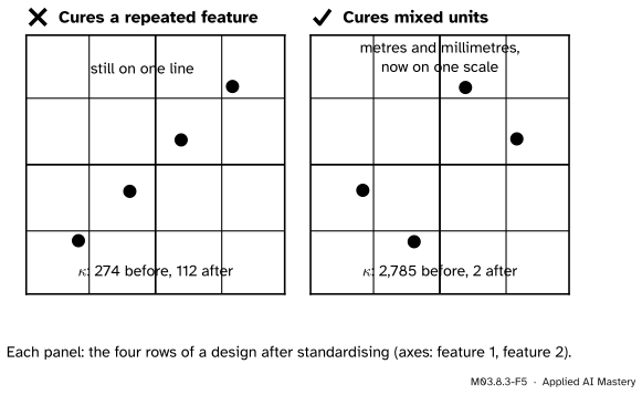
Remedy 1: standardise the features. Centre each column and divide it by its standard deviation. This cures ill-conditioning that comes from units: a column in millimetres beside one in metres has \(\kappa\) in the thousands for no real reason. It cannot cure a near-repeat, because two columns that are almost equal stay almost equal after the same kind of rescaling.
Remedy 2: work with an orthonormal basis (QR). Write \({\mat{A} = \mat{Q}\mat{R}}\) with orthonormal columns in \(\mat{Q}\) (M02.10.4). Multiplying \(\mat{R}\) by a matrix with orthonormal columns changes no singular value (the argument of exercise 2 of M03.8.2), so \(\mat{R}\) has the same singular values as \(\mat{A}\), and the fit solves \({\mat{R}\hat{\vect{x}} = \mat{Q}\T\vect{y}}\), a system with condition number \({\kappa(\mat{A})}\), not \({\kappa(\mat{A})^2}\). The fitted values \(\mat{Q}\mat{Q}\T\vect{y}\) use only \(\mat{Q}\), whose condition number is 1. QR stops the squaring; it cannot remove the near-repeat itself.
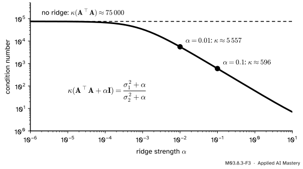
This is a spectral decomposition with eigenvalues \({\sigma_i^2 + \alpha}\), all positive. For a symmetric matrix with positive eigenvalues these are also its singular values, so the condition number is the largest over the smallest. Adding \(\alpha\) lifts the small end far more, in proportion, than the large end: the valley gets wider.
M03.8.3-F3
For the two-sensor design, the condition number of the ridge system falls from 75 000 to about 5 600 at \({\alpha = 0.01}\) and to about 600 at \({\alpha = 0.1}\).
The price is bias: ridge no longer solves the original least-squares problem. M03.7.4 shows which parts of the answer it shrinks.
Go deeper: where the Hilbert matrix comes from
Fit a polynomial \({c_1 + c_2 t + \dots + c_n t^{n-1}}\) to a function on \([0, 1]\) by least squares, with the integral \({\int_0^1 (\cdot)^2\,dt}\) in place of a sum of squares. The normal equations have the Gram matrix with entries \({\int_0^1 t^{i-1}t^{j-1}\,dt = 1/(i + j - 1)}\): the Hilbert matrix. On \([0, 1]\) the powers \(t^5\) and \(t^6\) have nearly the same shape, and the matrix records how alike all the powers are. A polynomial design on many evenly spread points is a sampled version of the same thing, which is why its line in the figure climbs the same way.
Worked example
Solve the two-sensor fit by hand, before and after the nudge.
The normal equations need \(\mat{A}\T\mat{A}\) and \(\mat{A}\T\vect{y}\). Since \({\vect{x}_1 \cdot \vect{x}_1 = 30}\), \({\vect{x}_1 \cdot \vect{x}_2 = 30}\) and \({\vect{x}_2 \cdot \vect{x}_2 = 30.0016}\), and \({\vect{y} = (2.02, 3.98, 5.98, 8.02)}\),
Subtract the first equation from the second: \({0.0016\,w_2 = 0.0016}\), so \({w_2 = 1}\), and then \({w_1 = 1}\). Now raise \(y_1\) from 2.02 to 2.12. The right side gains \({0.1\,(1, 1.02)}\) and becomes \({(60.1,\ 60.1036)}\). The same subtraction gives
\[
0.0016\,w_2 = 0.0036, \qquad w_2 = 2.25 ,
\]
and then \({w_1} = {(60.1 - 30 \times 2.25)/30} \approx {-0.247}\). All the information about how to split the weight sits in a difference of 0.0016 between two numbers near 60, and a nudge of 0.002 to that difference overwhelms it. The fitted values, though, move by at most 0.04.
With ridge, \({\alpha = 0.01}\) is added to both diagonal entries. Before the nudge the weights stay at about \({(1.00, 1.00)}\); after it they move only to about \({(0.91, 1.09)}\).
M03.8.3-F4
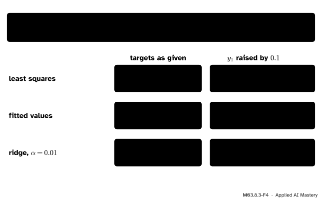
The worked example in one table. The coefficients swing; the predictions hardly move; ridge holds the coefficients still.
Code
The two-sensor fit, the three remedies, and the digit count, from scratch.
singular values: [7.74602 0.02828]  kappa(A): 273.9  kappa(A^T A): 75002
least squares: [1. 1.] -> [-0.247  2.25 ]  largest change in fitted values: 0.0383
ridge 0.01:    [1. 1.] -> [0.909 1.094]
Now the remedies, each measured by the condition number of the system it actually solves.
def standardise(X): centred = X - X.mean(axis=0)return centred / centred.std(axis=0, ddof=1)mixed = np.column_stack([x1, 1000* np.array([2.0, 1.0, 4.0, 3.0])]) # metres beside millimetresprint("standardise, mixed units: ", round(np.linalg.cond(mixed)), "->", round(np.linalg.cond(standardise(mixed)), 2))print("standardise, near-repeat: ", round(np.linalg.cond(A)), "->", round(np.linalg.cond(standardise(A))))Q, R = np.linalg.qr(A)print("normal equations solve with kappa =", round(np.linalg.cond(A.T @ A)), "; QR solves with kappa =", round(np.linalg.cond(R)))for alpha in [0.01, 0.1]: formula = (s[0] **2+ alpha) / (s[1] **2+ alpha)print(f"ridge alpha={alpha}: kappa = {np.linalg.cond(A.T @ A + alpha * np.eye(2)):.1f}, formula {formula:.1f}")
standardise, mixed units:   2785 -> 2.0
standardise, near-repeat:   274 -> 112
normal equations solve with kappa = 75002 ; QR solves with kappa = 274
ridge alpha=0.01: kappa = 5556.6, formula 5556.6
ridge alpha=0.1: kappa = 596.2, formula 596.2
Last, the digit count. Solve \({\mat{H}_n\vect{x} = \mat{H}_n\vect{1}}\), whose exact answer is all ones, and count the correct digits. The exact errors depend on the machine’s arithmetic library, so only their size is checked.
for n in [4, 6, 8, 10, 12]: H = hilbert(n) kappa = np.linalg.cond(H) x_hat = np.linalg.solve(H, H @ np.ones(n)) error =max(np.linalg.norm(x_hat -1) / np.sqrt(n), 1e-17) # never exactly zero, for the logprint(f"n={n:2d} kappa={kappa:8.1e} digits lost by the rule: {np.log10(kappa):4.1f}"f" digits correct: {-np.log10(error):4.1f}")
n= 4  kappa= 1.6e+04  digits lost by the rule:  4.2   digits correct: 13.5
n= 6  kappa= 1.5e+07  digits lost by the rule:  7.2   digits correct:  9.9
n= 8  kappa= 1.5e+10  digits lost by the rule: 10.2   digits correct:  7.1
n=10  kappa= 1.6e+13  digits lost by the rule: 13.2   digits correct:  3.4
n=12  kappa= 1.7e+16  digits lost by the rule: 16.2   digits correct:  1.0
The correct digits track \({16 - \log_{10}\kappa}\) within a digit or two, and by \({n = 12}\) almost nothing is left.
Explore
This module’s interactive, the condition explorer, lives in lesson M03.8.2. Press Nearly parallel: its two columns are a two-dimensional version of the two sensors, and the ellipse of solutions stretches along the same kind of valley.
Pitfalls
M03.8.3-F5
Wrong beside right. Standardising takes the mixed-units design from \({\kappa \approx 2785}\) to 2, but leaves the two sensors nearly on one line.
“Standardising the features fixes ill-conditioning.”
It fixes the kind that comes from units and scales. Two features that carry the same information still carry the same information after each is rescaled: the two-sensor design goes from \({\kappa \approx 274}\) only to 112. For a near-repeat, drop or merge a feature, or use ridge.
“A large condition number means the model predicts badly.”
The two-sensor fit predicts the training targets exactly and moves its predictions by at most 0.04 when a target moves by 0.1. What is unreliable is the split of the weight between the two features. That matters whenever the coefficients are read as explanations (“feature 1 lowers the answer”), and it is the instability that variance inflation measures in S03.
“To fit, invert \(\mat{A}\T\mat{A}\).”
Forming \(\mat{A}\T\mat{A}\) squares the condition number: 274 becomes 75 000, and the Hilbert-like designs above would lose every digit. Use np.linalg.lstsq or a QR factorisation, which work with \(\mat{A}\) itself, and never form an explicit inverse to solve a system.
Check yourself
Recall
1. Why do two nearly equal columns force a small singular value?
Show answer
The smallest singular value is the smallest stretch. The vector \({(1, -1)}\) (padded with zeros) subtracts the two columns, so its image is their tiny difference, and \(\sigma_n\) can be no larger than that stretch.
2. How fast does \({\kappa(\mat{H}_n)}\) grow?
Show answer
Exponentially, roughly like \(e^{3.5n}\): about 33 times larger for each extra column, from about \({4.8 \times 10^5}\) at \({n = 5}\) to about \({1.6 \times 10^{13}}\) at \({n = 10}\).
3. State the rule of thumb for the digits lost in solving a system.
Show answer
About \(\log_{10}\kappa\) of the roughly 16 significant digits of float64 are lost.
4. What is \({\kappa(\mat{A}\T\mat{A} + \alpha\mat{I})}\)?
5. Which cause of ill-conditioning does standardising cure, and which does it not?
Show answer
It cures features on very different scales or in different units. It does not cure features that nearly repeat one another.
Exercises
1.★ A design has columns \({(1, 0)}\) and \({(1, 0.01)}\). Use \({\sigma_1\sigma_2 = \abs{\det\mat{A}}}\) and \({\sigma_1^2 + \sigma_2^2 = \norm{\mat{A}}_F^2}\) to find its condition number, and estimate the digits lost.
Show solution
The determinant is \(0.01\) and \({\norm{\mat{A}}_F^2 = 1 + 1 + 0.0001 = 2.0001}\). The product of the singular values is tiny, so \({\sigma_1^2 \approx 2.0001}\), \({\sigma_1 \approx 1.4142}\) and \({\sigma_2 \approx 0.01/1.4142 \approx 0.00707}\). Then \({\kappa \approx 1.4142/0.00707 \approx 200}\), and about \({\log_{10}200 \approx 2.3}\) digits are lost. (The first identity holds because \({\det(\mat{A}\T\mat{A}) = \det(\mat{A})^2}\) is the product of the eigenvalues \(\sigma_1^2\sigma_2^2\).)
2.★★ For the two-sensor design, \({\sigma_1^2 \approx 60}\) and \({\sigma_2^2 = 0.0008}\). Find the smallest \(\alpha\) that makes \({\kappa(\mat{A}\T\mat{A} + \alpha\mat{I}) \le 100}\).
Show solution
We need \({(60 + \alpha)/(0.0008 + \alpha) \le 100}\), that is \({60 + \alpha \le 0.08 + 100\alpha}\), or \({99\alpha \ge 59.92}\). So \({\alpha \ge 0.605}\), roughly. The condition number falls quickly once \(\alpha\) passes \(\sigma_2^2\) and then slowly: reaching 100 needs an \(\alpha\) near one hundredth of \(\sigma_1^2\).
3.★★★ Two columns \(\vect{a}_i\) and \(\vect{a}_j\) of \(\mat{A}\) satisfy \({\norm{\vect{a}_i - \vect{a}_j} = \delta}\). Prove that \({\kappa(\mat{A}) \ge \sqrt2\,\sigma_1/\delta}\), and check it on the two-sensor design.
Show solution
Let \(\vect{z}\) have \({+1}\) in place \(i\), \({-1}\) in place \(j\) and zeros elsewhere. Then \({\mat{A}\vect{z} = \vect{a}_i - \vect{a}_j}\) and \({\norm{\vect{z}} = \sqrt2}\). The smallest stretch is at most this one: \({\sigma_n \le \delta/\sqrt2}\). Divide \(\sigma_1\) by both sides: \(\kappa = \sigma_1/\sigma_n \ge \sqrt2\,\sigma_1/\delta\). For the two sensors, \({\delta = 0.04}\) and \({\sigma_1 \approx 7.7460}\), so \(\kappa \ge 1.4142 \times 7.7460/0.04 \approx 273.86\). The true value is also 273.86 to two decimals (the bound is 273.863, the truth 273.865), so the bound is almost exact here.
Summary card
Features that nearly repeat make a long valley of almost equal fits, and a large \(\kappa\).
M03.8.3-F1
Same predictions, very different weights.
Near-repeat columns: \({\sigma_n} \le {\norm{\vect{a}_i - \vect{a}_j}/\sqrt2}\), so \(\kappa\) is large.
Hilbert and polynomial designs: \(\kappa\) grows exponentially, \({\kappa(\mat{H}_n) \sim e^{3.5n}}\).
About \(\log_{10}\kappa\) of 16 digits are lost.
Standardise for units; QR to avoid squaring; ridge: \({\kappa} = {(\sigma_1^2 + \alpha)/(\sigma_n^2 + \alpha)}\).
Sources and next steps
Sources. Each was opened and checked against this lesson on 15 November 2026.
Nicholas Higham, What is the Hilbert matrix? (2020): the entries \({1/(i + j - 1)}\), the growth \({\kappa_2(\mat{H}_n) \sim e^{3.5n}}\), and that \(\mat{H}_{12}\) is numerically singular in double precision.
SciPy reference, scipy.linalg.hilbert: hilbert(n) returns the \(n\) by \(n\) matrix with entries 1 / (i + j + 1), counting from zero.
NumPy reference, numpy.vander: vander(x, N) has N columns, powers decreasing from left to right unless increasing=True.
Cleve Moler, Numerical Computing with MATLAB, chapter 2, section 2.9: the computed solution’s relative error is at most about \({\rho\,\kappa(\mat{A})\,\varepsilon}\), with \(\rho\) rarely larger than about 10, the basis of the digits rule.