Solve the same least-squares problem by the normal equations, by QR and by the SVD. Derive the SVD formula, compare the cost of the three routes, and measure on a degree-10 polynomial fit how the normal equations lose about twice as many digits.
M03.7.2L2 Intermediate25 minIn review (what this means)
The maths and code on this page are checked by automated tests on every change, but an independent reader has not signed it off yet. Spot a mistake or a confusing step? Tell us.
Solve a least-squares problem by the normal equations, by QR and by the SVD, by hand on a 3 by 2 example.
Derive the SVD solution x-hat = V Sigma^(-1) U-transpose b from the normal equations.
Compare the cost of the three routes and explain why the normal equations lose about twice as many digits.
Use numpy.linalg.lstsq and scipy.linalg.lstsq and read everything they return.
The question
The last lesson ended with a formula, \(\hat{\vect{x}} = {(\mat{A}\T\mat{A})^{-1}\mat{A}\T\vect{b}}\), and with a library call, numpy.linalg.lstsq, that never forms \(\mat{A}\T\mat{A}\) at all. On paper they agree. Fit a degree-10 polynomial on a computer and the formula keeps about three correct digits while the library keeps about ten. Which routes are there to \(\hat{\vect{x}}\), what does each cost, and which one should a regression trust?
From the last lesson
1. What condition on the residual gives the normal equations?
Show answer
The residual \(\vect{e} = \vect{b} - \mat{A}\hat{\vect{x}}\) is perpendicular to every column: \(\mat{A}\T\vect{e} = \vect{0}\), which multiplies out to \(\mat{A}\T\mat{A}\hat{\vect{x}} = \mat{A}\T\vect{b}\).
2. What are the eigenvalues of the hat matrix \(\mat{H}\)?
Show answer
Only 1 (on the column space) and 0 (on the left null space), because \(\mat{H}^2 = \mat{H}\).
Intuition
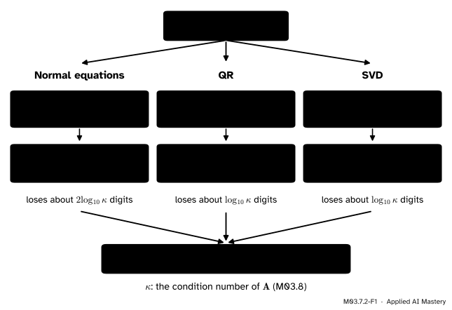
There are three standard routes from \(\mat{A}\) and \(\vect{b}\) to \(\hat{\vect{x}}\). Each factors something into easy pieces, then solves.
M03.7.2-F1
Three routes to one answer. In exact arithmetic they agree. On a computer, the route through \(\mat{A}\T\mat{A}\) loses about twice as many digits as the other two.
The difference is not in the algebra but in the rounding. A computer keeps about sixteen significant digits. A problem’s condition number\(\kappa(\mat{A}) = \sigma_1 / \sigma_n\), the largest singular value over the smallest (M03.5), measures how much it magnifies small errors; a useful rule of thumb, made precise in M03.8, is that about \(\log_{10}\kappa\) of the sixteen digits are lost. QR and the SVD work on \(\mat{A}\) itself. The normal equations first build \(\mat{A}\T\mat{A}\), whose condition number is \(\kappa(\mat{A})^2\), and so lose about \(2\log_{10}\kappa\) digits. When \(\kappa\) is \(10^7\), that is the difference between keeping nine digits and keeping two.
Build it up
Route 1: the normal equations. Form \(\mat{A}\T\mat{A}\) (an \(n \times n\) matrix) and \(\mat{A}\T\vect{b}\), then solve. Since \(\mat{A}\T\mat{A}\) is symmetric and positive definite when the columns are independent, Cholesky (M03.4.3) solves it cheaply. For an \(m \times n\) matrix this costs about \(mn^2\) arithmetic operations to form \(\mat{A}\T\mat{A}\) plus \(n^3/3\) for Cholesky: the cheapest of the three.
Route 2: QR. Factor \(\mat{A} = \mat{Q}\mat{R}\) (M02.10.4), with \(\mat{Q}\T\mat{Q} = \mat{I}\) and \(\mat{R}\) upper triangular and invertible. Put it into the normal equations. Since \({\mat{A}\T\mat{A}} = {\mat{R}\T\mat{Q}\T\mat{Q}\mat{R}} = {\mat{R}\T\mat{R}}\) and \(\mat{A}\T\vect{b} = {\mat{R}\T\mat{Q}\T\vect{b}}\):
The second line multiplies both sides on the left by \((\mat{R}\T)^{-1}\). One triangular solve, by back substitution, finishes the job. With Householder reflections the factorisation costs about \(2mn^2 - \tfrac23 n^3\) operations, roughly twice route 1 when \(m\) is much larger than \(n\).
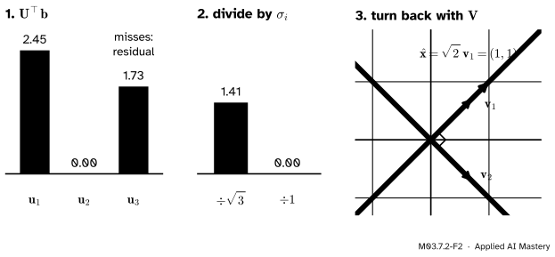
Route 3: the SVD. Take the thin SVD \(\mat{A} = \mat{U}\mat{\Sigma}\mat{V}\T\) (M03.5.3): \(\mat{U}\) is \(m \times n\) with orthonormal columns, \(\mat{\Sigma}\) is the \(n \times n\) diagonal of singular values, all positive when the columns are independent, and \(\mat{V}\) is \(n \times n\) orthogonal. The picture is three moves: read \(\vect{b}\) in the \(\vect{u}\)-directions, undo each stretch, turn back with \(\mat{V}\).
M03.7.2-F2
The SVD route on the running \(\mat{B}\) with \(\vect{b} = (3, 0, 0)\). The coordinate along \(\vect{u}_3\) lies outside the column space: no \(\hat{\vect{x}}\) can produce it, and it is the residual.
The formal statement
NoteThree formulas for one least-squares solution
If the \(m \times n\) matrix \(\mat{A}\) has independent columns, the least-squares solution of \(\mat{A}\vect{x} \approx \vect{b}\) is
So the normal equations read \(\mat{V}\mat{\Sigma}^2\mat{V}\T\hat{\vect{x}} = \mat{V}\mat{\Sigma}\mat{U}\T\vect{b}\). Undo the outer factors one at a time: multiply on the left by \(\mat{V}\T\) (using \(\mat{V}\T\mat{V} = \mat{I}\)), divide by the diagonal \(\mat{\Sigma}^2\), and multiply on the left by \(\mat{V}\) (using \(\mat{V}\mat{V}\T = \mat{I}\), since \(\mat{V}\) is square and orthogonal):
The residual. With the thin SVD, \(\mat{A}\hat{\vect{x}} = {\mat{U}\mat{U}\T\vect{b}}\), the sum of the shadows of \(\vect{b}\) on \(\vect{u}_1, \dots, \vect{u}_n\), so the hat matrix is \(\mat{H} = \mat{U}\mat{U}\T\), and what is left over is \(\vect{e}\).
Why the routes differ on a computer. In exact arithmetic the three lines are equal. A computed answer, though, is the exact answer to a slightly disturbed problem, and how far that moves \(\hat{\vect{x}}\) depends on the conditioning of the matrix that is actually solved. QR and the SVD solve with \(\mat{A}\)’s own factors and lose about \(\log_{10}\kappa(\mat{A})\) digits. The normal equations solve with \(\mat{A}\T\mat{A}\), whose singular values are \(\sigma_i^2\) (read off \(\mat{V}\mat{\Sigma}^2\mat{V}\T\) above), so
M03.8.2 makes the link between \(\kappa\) and lost digits precise; here we only measure it.
Go deeper: what the textbook error bounds say
Demmel’s lecture notes give the perturbation bound for least squares: the relative error in \(\hat{\vect{x}}\) is at most about \(\varepsilon\) times \({2\kappa/\cos\theta} + {\tan\theta\,\kappa^2}\), where \(\varepsilon \approx 2.2 \times 10^{-16}\) is the machine precision and \(\theta\) is the angle between \(\vect{b}\) and the column space. So when \(\vect{b}\) lies close to the column space (a good fit, small \(\theta\)) a stable method loses only about \(\log_{10}\kappa\) digits, and Householder QR and the SVD are such methods. For the normal equations, the notes say, “the error bound is always proportional to cond(A)^2, even when theta small”. For a good fit, then, the \(\kappa^2\) is a property of the route, not of the problem.
Worked example
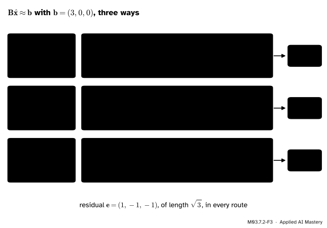
The running \(\mat{B}\), with columns \((1, 1, 0)\) and \((1, 0, 1)\), and \(\vect{b} = (3, 0, 0)\), three ways.
M03.7.2-F3
The three routes on one small problem. Each ends at \(\hat{\vect{x}} = (1, 1)\) with the same residual.
Normal equations.\(\mat{B}\T\mat{B} = \begin{bmatrix} 2 & 1 \\ 1 & 2 \end{bmatrix}\), the running \(\mat{S}\), and \(\mat{B}\T\vect{b} = (3, 3)\). The equations \(2x_1 + x_2 = 3\) and \(x_1 + 2x_2 = 3\) subtract to \(x_1 - x_2 = 0\), so \(x_1 = x_2 = 1\).
QR. The first column \((1, 1, 0)\) has length \(\sqrt{2}\), so \(r_{11} = \sqrt{2}\) and \(\vect{q}_1 = (1, 1, 0)/\sqrt{2}\). The second column has shadow \(r_{12} = {\vect{q}_1 \cdot (1, 0, 1)} = 1/\sqrt{2}\), and
of length \(r_{22} = \sqrt{3/2}\), so \(\vect{q}_2 = (1, -1, 2)/\sqrt{6}\). Then \(\mat{Q}\T\vect{b} = (3/\sqrt{2},\ 3/\sqrt{6})\). Back substitution: the bottom row gives \(x_2 = {(3/\sqrt{6})/\sqrt{3/2}} = 3/\sqrt{9} = 1\); the top row gives \({\sqrt{2}\,x_1} + {x_2/\sqrt{2}} = 3/\sqrt{2}\), so \(2x_1 + 1 = 3\) and \(x_1 = 1\).
SVD. From M03.5.3, \(\sigma_1 = \sqrt{3}\), \(\sigma_2 = 1\), \(\vect{u}_1 = (2, 1, 1)/\sqrt{6}\), \(\vect{u}_2 = (0, 1, -1)/\sqrt{2}\), \(\vect{v}_1 = (1, 1)/\sqrt{2}\) and \(\vect{v}_2 = (1, -1)/\sqrt{2}\). The coordinates are \(\vect{u}_1 \cdot \vect{b} = 6/\sqrt{6} = \sqrt{6}\) and \(\vect{u}_2 \cdot \vect{b} = 0\). Divide by the singular values, \(\sqrt{6}/\sqrt{3} = \sqrt{2}\) and \(0\), and turn back: \(\hat{\vect{x}} = \sqrt{2}\,\vect{v}_1 = (1, 1)\).
Residual.\({\mat{B}(1, 1)} = (2, 1, 1)\), so \(\vect{e} = (1, -1, -1)\), which is \(\sqrt{3}\) times the left null vector \(\vect{u}_3 = (1, -1, -1)/\sqrt{3}\) of M03.5.3. Its squared length, \(3\), is \(\norm{\vect{b}}^2\) minus the explained squares: \({9 - 6 - 0} = 3\).
Code
All three routes from scratch, on the running \(\mat{B}\) and on the four running points.
import numpy as npimport scipy.linalgdef by_normal_equations(A, b):return np.linalg.solve(A.T @ A, A.T @ b)def by_qr(A, b): Q, R = np.linalg.qr(A) # reduced: Q is m by n, R is n by nreturn scipy.linalg.solve_triangular(R, Q.T @ b)def by_svd(A, b): U, s, Vt = np.linalg.svd(A, full_matrices=False)return Vt.T @ ((U.T @ b) / s) # V Sigma^{-1} U^T bB = np.array([[1.0, 1.0], [1.0, 0.0], [0.0, 1.0]])b = np.array([3.0, 0.0, 0.0])A4 = np.column_stack([np.ones(4), [0.0, 3.0, 4.0, 7.0]])b4 = np.array([1.0, 2.0, 4.0, 5.0])for solve in (by_normal_equations, by_qr, by_svd):print(f"{solve.__name__:20s}", solve(B, b), solve(A4, b4))
Now the experiment of the hook: a degree-10 polynomial through 50 points on \([0, 1]\), with known coefficients (all ones), so that the error can be measured.
x = np.linspace(0.0, 1.0, 50)V = np.vander(x, 11, increasing=True) # columns 1, x, x^2, ..., x^10truth = np.ones(11)y = V @ truthkappa = np.linalg.cond(V)eps = np.finfo(float).epsdef digits_lost(estimate):return np.log10(np.linalg.norm(estimate - truth) / np.linalg.norm(truth) / eps)lost = {solve.__name__: digits_lost(solve(V, y)) for solve in (by_normal_equations, by_qr, by_svd)}print(f"kappa(V) = {kappa:.2e}, log10 kappa = {np.log10(kappa):.1f}")print(f"kappa(V^T V) = {np.linalg.cond(V.T @ V):.2e}, kappa(V)^2 = {kappa **2:.2e}")for name, d in lost.items():print(f"{name:20s} loses about {d:.1f} digits")
kappa(V) = 2.04e+07, log10 kappa = 7.3
kappa(V^T V) = 4.14e+14, kappa(V)^2 = 4.14e+14
by_normal_equations  loses about 12.9 digits
by_qr                loses about 5.7 digits
by_svd               loses about 5.5 digits
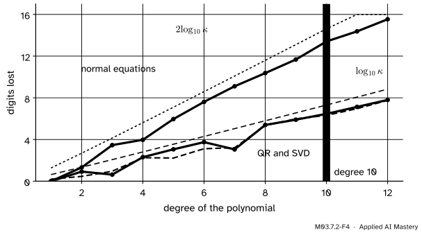
In the run above the normal equations lose about 13 digits and QR and the SVD about 6, against \(\log_{10}\kappa \approx 7.3\); the exact numbers vary a little between computers, the factor of about two does not. The plot below repeats the measurement for every degree from 1 to 12.
M03.7.2-F4
Digits lost by each route as the polynomial degree grows. The normal equations track \(2\log_{10}\kappa\); QR and the SVD track \(\log_{10}\kappa\). At degree 12 the normal equations have nothing left.
Last, the library. SciPy’s default driver is LAPACK’s gelsd, which computes “the minimum-norm solution … using the singular value decomposition (SVD) of A”. NumPy’s lstsq is SVD-based too: its cut-off is stated in terms of singular values, and it returns them.
sol, squares, rank, sing = np.linalg.lstsq(B, b)print("numpy:", sol, squares, rank, sing)sol2, residues, rank2, sing2 = scipy.linalg.lstsq(B, b)print("scipy:", sol2, residues, rank2, sing2)print("numpy on the polynomial loses", round(float(digits_lost(np.linalg.lstsq(V, y)[0])), 1), "digits")
Each returns four things: the solution, the sum of squared residuals (here \(3\)), the rank and the singular values \(\sqrt{3}\) and \(1\). NumPy treats a singular value as zero when it is smaller than rcond times the largest one, and the default rcond is the machine precision times \(\max(m, n)\).
Explore
The module’s interactive is in lesson M03.7.1. Every route of this lesson lands on the same foot of the perpendicular you see there; they differ only in how many digits of it they keep.
Pitfalls
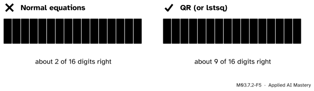
M03.7.2-F5
Wrong beside right, for the degree-10 polynomial fit: how many digits of the coefficients are right.
“np.linalg.inv(A.T @ A) @ A.T @ b is the formula, so it is the code.”
It is the formula for a blackboard. It squares the condition number, and inv adds rounding of its own. Use np.linalg.lstsq or scipy.linalg.lstsq, or QR. Austin’s text puts it plainly: the normal equations can let rounding errors accumulate, and QR is “numerically more reliable”.
“The residual is tiny, so the coefficients must be right.”
The normal-equations fit above has a relative residual below \(10^{-7}\) and still only about three correct digits in its coefficients. With nearly dependent columns many different coefficient vectors make almost the same predictions, so a small residual says little about the coefficients. Lesson M03.7.4 returns to this.
“The second output of lstsq is the residual vector.”
It is the sum of squared residuals, \(\norm{\vect{e}}^2\). NumPy returns it as an array of length 1 for a single right-hand side, and as an empty array when the rank is below \(n\) or \(m \le n\). Compute b - A @ x for the vector itself.
Check yourself
Recall
1. Write the least-squares solution by QR and by the SVD.
Show answer
\(\mat{R}\hat{\vect{x}} = \mat{Q}\T\vect{b}\), solved by back substitution, and \(\hat{\vect{x}} = \mat{V}\mat{\Sigma}^{-1}\mat{U}\T\vect{b}\).
2. What does \(\mat{A}\T\mat{A}\) become in terms of the SVD of \(\mat{A}\)?
Show answer
\(\mat{V}\mat{\Sigma}^2\mat{V}\T\): the same right singular vectors, with the singular values squared.
3. Which route is cheapest, and what is its rough cost?
Show answer
The normal equations: about \(mn^2\) operations to form \(\mat{A}\T\mat{A}\) and \(n^3/3\) for Cholesky. Householder QR costs about \(2mn^2 - \tfrac23 n^3\).
4. About how many digits does each route lose, in terms of \(\kappa(\mat{A})\)?
Show answer
QR and the SVD about \(\log_{10}\kappa\); the normal equations about \(2\log_{10}\kappa\), because \(\kappa(\mat{A}\T\mat{A}) = \kappa(\mat{A})^2\).
5. What four things does numpy.linalg.lstsq return?
Show answer
The solution, the sums of squared residuals (empty when the rank is below \(n\) or \(m \le n\)), the rank, and the singular values.
Exercises
1.★ M02.10.4 found \(\mat{R} = \begin{bmatrix} 2 & 7 \\ 0 & 5 \end{bmatrix}\) for the four running points. Compute \(\mat{R}\T\mat{R}\) and compare it with the \(\mat{A}\T\mat{A}\) of lesson M03.7.1.
which is \(\mat{A}\T\mat{A}\), as \({\mat{A}\T\mat{A}} = {\mat{R}\T\mat{Q}\T\mat{Q}\mat{R}} = {\mat{R}\T\mat{R}}\) says. The triangle \(\mat{R}\) is the Cholesky factor of \(\mat{A}\T\mat{A}\), found without ever forming it.
2.★★ Solve \(\mat{B}\vect{x} \approx \vect{b}\) for \(\vect{b} = (0, 1, -1)\) by the SVD route, and check by the normal equations. What is the residual, and why?
Show solution
\(\vect{u}_1 \cdot \vect{b} = {(0 + 1 - 1)/\sqrt{6}} = 0\) and \(\vect{u}_2 \cdot \vect{b} = {(0 + 1 + 1)/\sqrt{2}} = \sqrt{2}\). Dividing by \(\sigma_1 = \sqrt{3}\) and \(\sigma_2 = 1\) gives \(0\) and \(\sqrt{2}\), so \(\hat{\vect{x}} = {\sqrt{2}\,\vect{v}_2} = (1, -1)\). Check: \(\mat{B}\T\vect{b} = (1, -1)\) and \(\mat{S}^{-1} = \tfrac13\begin{bmatrix} 2 & -1 \\ -1 & 2 \end{bmatrix}\), so \(\hat{\vect{x}} = \tfrac13(2 + 1,\ -1 - 2) = (1, -1)\). Then \(\mat{B}(1, -1) = (0, 1, -1) = \vect{b}\), so the residual is \(\vect{0}\): \(\vect{b} = \sqrt{2}\,\vect{u}_2\) already lies in the column space, and \(\vect{u}_3 \cdot \vect{b} = {(0 - 1 + 1)/\sqrt{3}} = 0\).
3.★★★ Using the full SVD, prove that \(\norm{\vect{e}}^2 = {\norm{\vect{b}}^2} - \sum_{i=1}^{n} (\vect{u}_i \cdot \vect{b})^2\) for a matrix with independent columns. Check it on \(\vect{b} = (3, 0, 0)\).
Show solution
The full \(\mat{U}\) is \(m \times m\) orthogonal, so its columns \(\vect{u}_1, \dots, \vect{u}_m\) are an orthonormal basis of \(\R^m\) and \(\vect{b} = \sum_{i=1}^{m} (\vect{u}_i \cdot \vect{b})\,\vect{u}_i\), with \(\norm{\vect{b}}^2 = \sum_{i=1}^{m} (\vect{u}_i \cdot \vect{b})^2\) by Pythagoras. The projection is \(\mat{A}\hat{\vect{x}} = \mat{U}_n\mat{U}_n\T\vect{b}\), the first \(n\) terms, so
and \(\norm{\vect{e}}^2 = \sum_{i>n} (\vect{u}_i \cdot \vect{b})^2\), which is \(\norm{\vect{b}}^2\) minus the first \(n\) squares. For \(\mat{B}\) and \(\vect{b} = (3, 0, 0)\): \(9 - 6 - 0 = 3 = (\vect{u}_3 \cdot \vect{b})^2 = (\sqrt{3})^2\), the squared length of \(\vect{e} = (1, -1, -1)\).
Summary card
Three routes, one answer; trust the ones that do not square \(\kappa\).
M03.7.2-F1
Normal equations, QR, SVD.
Normal equations.\(\mat{A}\T\mat{A}\hat{\vect{x}} = \mat{A}\T\vect{b}\): cheapest, \(\kappa^2\).
QR.\(\mat{R}\hat{\vect{x}} = \mat{Q}\T\vect{b}\): about twice the work, \(\kappa\).
SVD.\(\hat{\vect{x}} = \sum_i (\vect{u}_i \cdot \vect{b}/\sigma_i)\,\vect{v}_i\): the most complete.
In code.np.linalg.lstsq and scipy.linalg.lstsq, both SVD-based.
Sources and next steps
Sources. Each was opened and checked against this lesson on 15 November 2026.
James Demmel, Math 221 lecture 7 notes, University of California, Berkeley, spring 2022. The operation counts \(mn^2 + n^3/3\) for the normal equations and \(2n^2m - \tfrac23 n^3\) for Householder QR; the perturbation bound with \({2\kappa/\cos\theta} + {\tan\theta\,\kappa^2}\); the remark that for the normal equations “the error bound is always proportional to cond(A)^2”; and the summary that the SVD gives the most complete answer and is best when \(\mat{A}\) is ill-conditioned.
David Austin, Understanding Linear Algebra: Section 6.5, Orthogonal least squares, subsection Using QR factorizations, which calls the QR route “numerically more reliable”; and Section 7.5, Using Singular Value Decompositions, subsection Least-squares problems (Proposition 7.5.3), the solution \(\mat{V}_r\mat{\Sigma}_r^{-1}\mat{U}_r\T\vect{b}\).
NumPy, numpy.linalg.lstsq (the four outputs, when the residuals are empty, and the default rcond) and numpy.linalg.qr (the default mode 'reduced').
SciPy, scipy.linalg.lstsq. The drivers 'gelsd' (the default), 'gelsy' and 'gelss', and the outputs.
LAPACK, DGELSD. “DGELSD computes the minimum-norm solution to a real linear least squares problem … using the singular value decomposition (SVD) of A.”
Next.M03.7.3 The pseudoinverse asks what happens when the columns are dependent and the normal equations have infinitely many solutions.