Find the dominant eigenvector of a matrix by multiplying and rescaling, again and again. Derive why it converges at the rate of the ratio of the two largest eigenvalues, estimate the eigenvalue with the Rayleigh quotient, and meet the three ways it fails.
M03.2.4L2 Intermediate25 minIn review (what this means)
The maths and code on this page are checked by automated tests on every change, but an independent reader has not signed it off yet. Spot a mistake or a confusing step? Tell us.
Run the power method by hand: multiply by the matrix, rescale to length 1, repeat.
Derive from the eigen-expansion that the error shrinks by the factor |lambda_2 / lambda_1| per step.
Estimate the dominant eigenvalue with the Rayleigh quotient x-transpose A x / x-transpose x.
Recognise the three failures: no component along v_1, two eigenvalues of equal size, and complex eigenvalues.
Implement the method with a stopping rule and check it against numpy.linalg.eig.
The question
Google ranks web pages by the dominant eigenvector of a matrix with billions of rows. Nobody can write down its characteristic polynomial, let alone solve it. Yet one eigenvector is found every time, by an algorithm that only multiplies a vector by the matrix. How can multiplying alone find an eigenvector, and how fast does it get there?
From the last lesson
1. What are the eigenvalues and eigenvectors of \(\mat{F} = \begin{bmatrix} 1 & 1 \\ 1 & 0 \end{bmatrix}\)?
Show answer
\(\varphi = {(1 + \sqrt5)/2}\) and \(\psi = {(1 - \sqrt5)/2} = -1/\varphi\), with eigenvectors \((\varphi, 1)\) and \((\psi, 1)\).
2. At what rate does \(F_{k+1}/F_k\) approach \(\varphi\)?
Show answer
The error shrinks by the factor \(\abs{\psi/\varphi} = 1/\varphi^2 \approx 0.382\) at each step, changing sign each time.
Intuition
The last lesson watched the Fibonacci states line up along the eigenvector of the larger eigenvalue. That was no accident. Apply any matrix again and again, and the eigen-coordinate with the largest eigenvalue grows fastest, so the vector turns towards that eigenvector.
The lengths blow up (or shrink to nothing), which a computer cannot store for long. But only the direction matters. So after every multiplication, rescale the vector back to length 1. That is the power method: multiply, rescale, repeat.
M03.2.4-F1
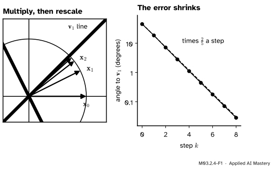
The power method on the running matrix \(\mat{A}\) from \(\vect{x}_0 = (1, 0)\). Every iterate has length 1 and points closer to \(\vect{v}_1 = (1, 1)\). On a log scale the angle to \(\vect{v}_1\) falls in a straight line: it is multiplied by about \(\frac25\) at every step.
The eigenvalues of \(\mat{A}\) are 5 and 2, and \(\tfrac25\) is their ratio. The rest of the lesson shows why the ratio is the speed.
Build it up
Step 1. One step, in three frames.
M03.2.4-F2
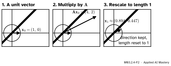
One step of the power method. Multiplying by \(\mat{A}\) turns the vector towards \(\vect{v}_1\) and makes it longer; rescaling keeps only the new direction.
\(\mat{A}(1, 0) = (4, 2)\), of length \(\sqrt{20} \approx 4.472\), so \(\vect{x}_1 = {(4, 2)/\sqrt{20}} \approx (0.894, 0.447)\).
Step 2. Rescaling does not change the direction of later steps. Multiplying by a matrix is linear, so \(\mat{A}(s\vect{x}) = s\,\mat{A}\vect{x}\) for any number \(s\). Rescaling only changes the lengths, so \(\vect{x}_k\) is \(\mat{A}^k\vect{x}_0\) rescaled to length 1. We may study the plain powers \(\mat{A}^k\vect{x}_0\) and rescale at the end.
Step 3. Write the start in eigen-coordinates. From lesson M03.2.2, \((1, 0) = {\tfrac23\vect{v}_1 + \tfrac13\vect{v}_2}\), so
The number in front only sets the length, which rescaling throws away. Inside the bracket, the \(\vect{v}_2\) part is \(\tfrac12(\tfrac25)^k\): one half, then 0.2, then 0.08, 0.032, and so on. It is multiplied by exactly \(\tfrac25\) at every step. That ratio, the size of the \(\vect{v}_2\) part compared with the \(\vect{v}_1\) part, is the error.
The formal statement
NoteResult: convergence of the power method
Let \(\mat{A}\) be diagonalisable with eigenvalues ordered by size, \(\abs{\lambda_1} > \abs{\lambda_2} \ge \dots \ge \abs{\lambda_n}\), and let the start \(\vect{x}_0 = c_1\vect{v}_1 + \dots + c_n\vect{v}_n\) have \(c_1 \neq 0\). Then the direction of \(\mat{A}^k\vect{x}_0\) approaches the line of \(\vect{v}_1\), and its distance from that line, measured by the eigen-coordinates, shrinks like \(\abs{\lambda_2/\lambda_1}^k\).
Derivation. By the vector form of lesson M03.2.2, then taking out \(c_1\lambda_1^k\), which is not zero:
For every \(j \ge 2\), \(\abs{\lambda_j/\lambda_1} \le \abs{\lambda_2/\lambda_1} < 1\), so each term of the sum is at most a fixed number times \(\abs{\lambda_2/\lambda_1}^k\) and goes to \(\vect{0}\). The bracket tends to \(\vect{v}_1\), and rescaling to length 1 removes the factor \(c_1\lambda_1^k\) (up to its sign). \(\blacksquare\)
Two remarks. If \(\lambda_1 < 0\), the factor \(\lambda_1^k\) changes sign each step, so the rescaled vectors flip between \(\vect{v}_1/\norm{\vect{v}_1}\) and its negative: the line converges. And the rate depends only on the ratio: eigenvalues 5 and 2 give the same speed as 500 and 200.
The eigenvalue estimate. Once \(\vect{x}\) is close to an eigenvector, \(\mat{A}\vect{x}\) is close to \(\lambda_1\vect{x}\), and the number that best matches them is the Rayleigh quotient
For an exact eigenvector it gives the eigenvalue exactly: \(\vect{x}\T(\lambda\vect{x}) / \vect{x}\T\vect{x} = \lambda\). For a nearly exact one it gives a nearly exact eigenvalue. (For symmetric matrices it has a stronger property, the subject of lesson M03.3.4.)
A stopping rule. We do not know \(\vect{v}_1\), so we cannot measure the error directly. Instead stop when two successive iterates (with signs matched) differ by less than a tolerance, say \(\norm{\vect{x}_{k+1} - \vect{x}_k} < 10^{-10}\). Because the error shrinks by a constant factor, the change from one step to the next shrinks at the same rate.
Go deeper: symmetric matrices converge twice as fast in the eigenvalue
For a symmetric matrix the eigenvectors can be chosen perpendicular and of length 1 (module M03.3). Write \(\vect{x} = \vect{q}_1 + \varepsilon\vect{q}_2\) with small \(\varepsilon\). Then \(\mat{S}\vect{x} = \lambda_1\vect{q}_1 + \varepsilon\lambda_2\vect{q}_2\), and the cross terms vanish because \(\vect{q}_1 \cdot \vect{q}_2 = 0\):
So \(\lambda_1 - R(\vect{x}) = {\varepsilon^2(\lambda_1 - \lambda_2)/(1 + \varepsilon^2)}\): an error of size \(\varepsilon\) in the vector gives an error of size \(\varepsilon^2\) in the eigenvalue, which therefore shrinks like \(\abs{\lambda_2/\lambda_1}^{2k}\). For \(\mat{S} = \begin{bmatrix} 2 & 1 \\ 1 & 2 \end{bmatrix}\) from \((1, 0)\), the errors in the estimate of 3 are \(1, 0.2, 0.024, 0.0027, \dots\); after the first step each is about \(\tfrac19 = (\tfrac13)^2\) of the one before. For the non-symmetric \(\mat{A}\) the cross terms do not vanish, and the estimate improves only at the rate \(\tfrac25\) of the vector.
Worked example
Run five steps of the power method on \(\mat{A}\) from \(\vect{x}_0 = (1, 0)\), tracking the angle to \(\vect{v}_1\) and the Rayleigh quotient.
By hand, rescaling can wait (Step 2 above): multiply by \(\mat{A}\) five times and rescale each vector only to read it.
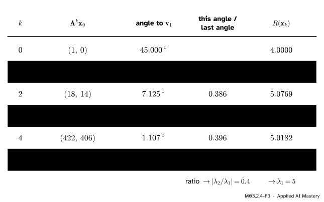
Two more steps give \((422, 406)\) and \((2094, 2062)\), the first column of \(\mat{A}^5\) from lesson M03.2.2. For the Rayleigh quotient of \(\vect{x} = (4, 2)\): \(\mat{A}\vect{x} = (18, 14)\), so \(\vect{x}\T\mat{A}\vect{x} = {72 + 28} = 100\) and \(\vect{x}\T\vect{x} = 20\), giving \(R = 5\) (a lucky exact hit). For \((18, 14)\): \(\mat{A}\vect{x} = (86, 78)\), so \(R = {(1548 + 1092)/(324 + 196)} = {2640/520} \approx 5.0769\).
M03.2.4-F3
Five steps on the running matrix. The angle to \(\vect{v}_1\) shrinks by a factor that settles at \(|\lambda_2/\lambda_1| = 0.4\), and the Rayleigh quotient closes in on \(\lambda_1 = 5\).
The angle ratios \(0.410, 0.386, 0.392, 0.396, 0.399\) approach \(0.4\), as the derivation predicted. The eigen-coordinate ratio of Step 4 shrinks by exactly 0.4: it is \(0.5, 0.2, 0.08, 0.032, 0.0128,
0.00512\). The angle is a slightly bent measure of the same thing, which is why its ratio only approaches 0.4.
Code
From scratch, with the stopping rule.
import numpy as npdef power_method(M, x0, tol=1e-10, max_steps=1000):"""Dominant eigenvector (length 1), Rayleigh estimate and the number of steps used.""" x = np.asarray(x0, dtype=float) x = x / np.linalg.norm(x)for step inrange(1, max_steps +1): y = M @ x y = y / np.linalg.norm(y)if y @ x <0: # match signs, so a negative lambda_1 does not look like a change y =-yif np.linalg.norm(y - x) < tol:return y, y @ M @ y, step x = yreturn x, x @ M @ x, max_steps # no convergence within max_stepsA = np.array([[4.0, 1.0], [2.0, 3.0]])v, lam, steps = power_method(A, [1.0, 0.0])print("eigenvector:", v, " estimate:", lam, " steps:", steps)
The rule stops after 26 steps: the change between iterates is about \({1.3 \times 10^{-10}}\) at step 25 and \({5 \times 10^{-11}}\) at step 26. That fits the rate, since \(0.4^{25} \approx 10^{-10}\). Now the same matrix through the library, and the symmetric \(\mat{S}\) and the Fibonacci matrix through our function:
\(\mat{S}\), with ratio \(\tfrac13\), and \(\mat{F}\), with ratio about 0.382, both need fewer steps than \(\mat{A}\), with ratio 0.4. A smaller ratio means faster convergence.
Explore
This module’s interactive, the power stepper, lives in lesson M03.2.2. Switch on normalise each step and press step a few times with the running matrix \(\mat{A}\): the read-out gives the angle to the dominant eigenvector and the ratio \(|\lambda_2/\lambda_1| = 0.40\). Then try the swap matrix, whose ratio is 1: the angle never shrinks. Last, try the map \(\mat{T}\), which has no real eigen-line at all, so the vector keeps turning.
Pitfalls
M03.2.4-F4
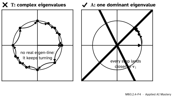
Wrong beside right. The running map \(\mat{T}\) of M02 has complex eigenvalues of equal size, so the power method turns round the circle for ever. \(\mat{A}\) has one eigenvalue larger than the other, and the iterates settle.
“The power method finds an eigenvector of every matrix.”
It needs one eigenvalue strictly larger in size than all the others. The map \(\mat{T} = \begin{bmatrix} 1 & 1 \\ -1 & 2 \end{bmatrix}\) has eigenvalues \({\tfrac32 \pm \tfrac{\sqrt3}{2}i}\), both of size \(\sqrt3\) (lesson M03.1.4). In a suitable basis it turns by 30 degrees and stretches, so the iterates keep turning and never settle.
M03.2.4-F5
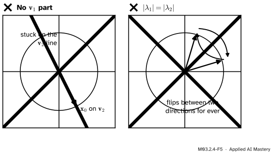
Two more ways to fail. A start with no component along \(\vect{v}_1\) never finds it (in exact arithmetic). Two eigenvalues of equal size, here 1 and \(-1\), leave the iterates flipping between two directions.
“Any start will do.”
Almost any. If \(c_1 = 0\), the \(\vect{v}_1\) term is missing from the start and from every iterate. Start \(\mat{A}\)’s method at \((1, -2)\), which is \(\vect{v}_2\), and every iterate is \(\vect{v}_2\) again; our stopping rule even reports convergence after one step, to the eigenvalue 2. In floating point, rounding usually plants a tiny \(\vect{v}_1\) part that eventually grows, but you cannot count on it. A random start has \(c_1 = 0\) with probability zero, which is why libraries start randomly.
“Two eigenvalues of equal size are a tie, so either eigenvector is found.”
Neither is. For the swap matrix \(\begin{bmatrix} 0 & 1 \\ 1 & 0 \end{bmatrix}\), with eigenvalues 1 and \(-1\), the ratio is 1: the \(\vect{v}_2\) part never shrinks relative to the \(\vect{v}_1\) part, and its sign flips every step, so the iterates alternate between two directions. A ratio close to 1 is nearly as bad: convergence becomes very slow.
Check yourself
Recall
1. What are the two moves of one step of the power method?
Show answer
Multiply the current vector by the matrix, then rescale the result to length 1.
2. What sets the speed of convergence?
Show answer
The ratio \(\abs{\lambda_2/\lambda_1}\) of the second-largest to the largest eigenvalue size: the error is multiplied by about that factor at each step.
3. How is the eigenvalue estimated from an iterate \(\vect{x}\)?
Show answer
By the Rayleigh quotient \(R(\vect{x}) = \vect{x}\T\mat{A}\vect{x} / \vect{x}\T\vect{x}\).
4. For the running matrix from \((1, 0)\), by what factor does the eigen-coordinate ratio shrink, and where do the iterates end up?
Show answer
By exactly \(\tfrac25\) each step, from \(\tfrac12\) to \(0.2\) to \(0.08\) and so on, and the iterates approach \((1, 1)/\sqrt2\), with \(R\) approaching 5.
5. Name the three situations in which the power method fails.
Show answer
A start with no component along \(\vect{v}_1\); two eigenvalues of the same largest size (such as 1 and \(-1\)); and complex eigenvalues, such as those of the running map \(\mat{T}\).
Exercises
1.★ Run two steps of the power method by hand on \(\mat{S} = \begin{bmatrix} 2 & 1 \\ 1 & 2 \end{bmatrix}\) from \((1, 0)\), without rescaling, and compute the Rayleigh quotient of the result.
Show solution
\(\mat{S}(1, 0) = (2, 1)\) and \({\mat{S}(2, 1)} = {(4 + 1,\; 2 + 2)} = (5, 4)\). For \(\vect{x} = (5, 4)\), \(\mat{S}\vect{x} = {(10 + 4,\; 5 + 8)} = (14, 13)\), so \(\vect{x}\T\mat{S}\vect{x} = {70 + 52} = 122\) and \(\vect{x}\T\vect{x} = {25 + 16} = 41\), giving \(R = 122/41 \approx 2.9756\), already close to the dominant eigenvalue 3.
2.★★ On \(\mat{A}\) from \((1, 0)\), the eigen-coordinate ratio after \(k\) steps is \(\tfrac12(0.4)^k\). How many steps make it smaller than \(10^{-6}\)?
Show solution
We need \(\tfrac12(0.4)^k < 10^{-6}\), that is, \(0.4^k < {2 \times 10^{-6}}\). Take logarithms; since \(\ln 0.4 < 0\), dividing flips the inequality:
So 15 steps. Check: \(\tfrac12(0.4)^{14} \approx {1.3 \times 10^{-6}}\) and \(\tfrac12(0.4)^{15} \approx {5.4 \times 10^{-7}}\).
3.★★★ A shift replaces \(\mat{A}\) by \(\mat{A} - s\mat{I}\), which has the same eigenvectors and eigenvalues \(5 - s\) and \(2 - s\). For which \(s\) is \(5 - s\) still the dominant eigenvalue, what is the convergence ratio, and which shift is best? Check the best one directly.
Show solution
\({(\mat{A} - s\mat{I})\vect{v}} = {\mat{A}\vect{v} - s\vect{v}} = {(\lambda - s)\vect{v}}\), so the eigenvectors stay and the eigenvalues move by \(s\). \(5 - s\) dominates when \(\abs{5 - s} > \abs{2 - s}\), that is, when \(s\) is nearer to 2 than to 5: \(s < 3.5\). The ratio is then \(\abs{2 - s}/\abs{5 - s}\), which is 0 at \(s = 2\). Directly, \(\mat{A} - 2\mat{I} = \begin{bmatrix} 2 & 1 \\ 2 & 1 \end{bmatrix}\) sends every vector \((x, y)\) to \({(2x + y)}\,(1, 1)\): one step lands on \(\vect{v}_1\) exactly, unless \(2x + y = 0\), which is a start along \(\vect{v}_2\). A good shift needs the eigenvalue \(2\) in advance, which is why shifts are refined as the iteration runs in the better algorithms of module M10.5.
Summary card
Multiply and rescale: the largest eigenvalue takes over, at the speed of the eigenvalue ratio.
Sources. Each was opened and checked against this lesson on 15 November 2026.
David Austin, Understanding Linear Algebra, section Finding eigenvectors numerically (open textbook). The power method as the sequence \(x_{k+1} = Ax_k\) with each vector rescaled, the multipliers approaching the dominant eigenvalue, the warning that a start equal to \(v_2\) does not detect \(v_1\), and that matrices with repeated or complex eigenvalues need a modified method.
Wikipedia, Power iteration. Convergence is geometric with ratio \(\abs{\lambda_2/\lambda_1}\), the start must have a non-zero component along the dominant eigenvector, the Rayleigh quotient gives the eigenvalue, and the method is used to compute Google’s PageRank.
Gilbert Strang, Diagonalization and powers of A, MIT OpenCourseWare 18.06SC, lecture summary. The expansion \(u_k = A^ku_0 = c_1\lambda_1^kx_1 + \dots + c_n\lambda_n^kx_n\) on which the derivation rests.
NumPy reference, numpy.linalg.eig, used to check the result: eigenvalues in no particular order, with unit-length eigenvectors as columns.
Next. The power method is the engine of PageRank in module M03.9, and better eigenvalue algorithms, with shifts and many vectors at once, are in module M10.5. Module M03.3 turns to symmetric matrices, whose eigenvectors are perpendicular.