Multiply out S = Q Lambda Q-transpose and a symmetric matrix falls apart into a weighted sum of projections onto perpendicular lines. Use the pieces to act on a vector, to build S inverse, S to a power and the square root of S, and to glimpse low-rank approximation.
M03.3.3L2 Intermediate25 minIn review (what this means)
The maths and code on this page are checked by automated tests on every change, but an independent reader has not signed it off yet. Spot a mistake or a confusing step? Tell us.
Derive S = lambda_1 q_1 q_1-transpose + … + lambda_n q_n q_n-transpose by multiplying Q Lambda Q-transpose column by row.
Explain why each piece q q-transpose is the projection onto a line, and compute S x by projecting, scaling and adding.
Compute S inverse, a power of S and the square root of S by applying the function to the eigenvalues only.
Explain why dropping the pieces with small eigenvalues gives a good approximation of lower rank.
The question
The last lesson wrote a symmetric matrix as three factors. A data scientist often wants something else: the inverse of a covariance matrix for a distance, its square root to whiten data, a high power for a long chain of steps, or a cheap copy that keeps only what matters. Is there one view of a symmetric matrix that makes all of these easy?
From the last lesson
1. State the spectral theorem.
Show answer
Every real symmetric matrix is \(\mat{S} = \mat{Q}\mat{\Lambda}\mat{Q}\T\), with \(\mat{Q}\) orthogonal (orthonormal eigenvectors as columns) and \(\mat{\Lambda}\) the real diagonal matrix of eigenvalues.
2. What does a symmetric 2 by 2 matrix with eigenvalues 3 and 1 do to the unit circle?
Show answer
It makes an ellipse with half-widths 3 and 1 along the two eigenvectors.
Intuition
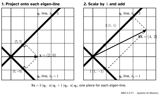
To apply \(\mat{S}\) to a vector, you do not need its entries at all. Drop the vector at right angles onto each eigen-line, stretch each shadow by its eigenvalue, and add the results.
M03.3.3-F1
\(\mat{S}\) applied to \(\vect{x} = {(2, 0)}\) without its entries: project onto the two eigen-lines, scale the shadows by 3 and 1, add. The answer is \({(4, 2)}\), which is twice the first column of \(\mat{S}\), as it must be.
Each eigen-line contributes one piece, and the pieces never interfere, because the lines are perpendicular. That splitting is what this lesson writes as a sum of matrices.
Build it up
Step 1. A shadow is a matrix. Lesson M02.3.4 found the projection of \(\vect{x}\) onto the line of a unit vector \(\vect{q}\): \({(\vect{q} \cdot \vect{x})\,\vect{q}}\). Write the dot product as \({\vect{q}\T\vect{x}}\) and move the number to the other side of the vector:
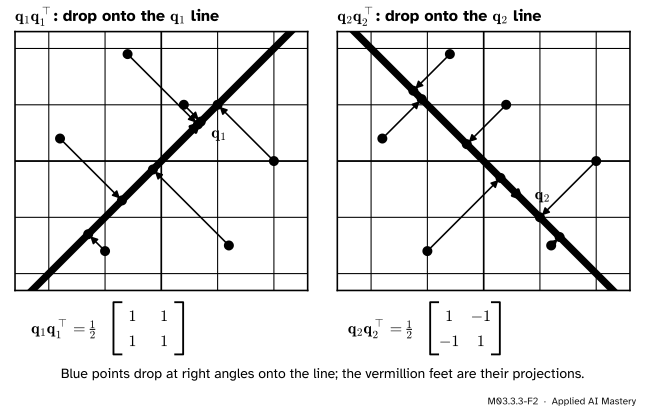
The column \(\vect{q}\) times the row \(\vect{q}\T\) is a square matrix, the outer product\(\vect{q}\vect{q}\T\). It is the projection onto the line of \(\vect{q}\).
Step 2. What the piece looks like. For \(\vect{q}_1 = {(1, 1)/\sqrt{2}}\), entry \(ij\) of \(\vect{q}_1\vect{q}_1\T\) is \({(q_1)_i (q_1)_j} = {\tfrac12}\), so \(\vect{q}_1\vect{q}_1\T = \tfrac12\begin{bmatrix} 1 & 1 \\ 1 & 1 \end{bmatrix}\). For \(\vect{q}_2 = {(1, -1)/\sqrt{2}}\) it is \(\tfrac12\begin{bmatrix} 1 & -1 \\ -1 & 1 \end{bmatrix}\). Each has rank one: every column is a multiple of \(\vect{q}\).
M03.3.3-F2
The two pieces of \(\mat{S}\) as maps. Each one drops every point of the plane onto its own line.
Step 3. Three facts about the pieces. Write \(\mat{P}_i = \vect{q}_i\vect{q}_i\T\).
Doing it twice changes nothing:\({\mat{P}_i\mat{P}_i} = {\vect{q}_i(\vect{q}_i\T\vect{q}_i)\vect{q}_i\T} = \mat{P}_i\), because \({\vect{q}_i\T\vect{q}_i} = 1\).
Two different pieces kill each other: for \({i \neq j}\), \({\mat{P}_i\mat{P}_j} = {\vect{q}_i(\vect{q}_i\T\vect{q}_j)\vect{q}_j\T} = \mat{0}\), because \({\vect{q}_i\T\vect{q}_j} = 0\).
All of them together do nothing:\({\mat{P}_1 + \cdots + \mat{P}_n} = {\mat{Q}\mat{Q}\T} = \mat{I}\), which is the next section’s expansion with every \(\lambda_i = 1\).
The formal statement
NoteThe spectral decomposition as a sum
If \(\mat{S} = \mat{Q}\mat{\Lambda}\mat{Q}\T\) with orthonormal eigenvectors \(\vect{q}_i\), then
and for every vector \(\vect{x}\), \(\mat{S}\vect{x} = {\sum_i \lambda_i\,(\vect{q}_i \cdot \vect{x})\,\vect{q}_i}\).
Derivation. A product of matrices can be expanded column by row: if \(\mat{B}\) has columns \(\vect{b}_k\) and \(\mat{C}\) has rows \(\vect{c}_k\T\), then \(\mat{B}\mat{C} = {\sum_k \vect{b}_k\vect{c}_k\T}\). Entry \(ij\) of the right-hand side is \({\sum_k (\vect{b}_k)_i(\vect{c}_k)_j} = {\sum_k b_{ik}c_{kj}}\), which is the row-times-column rule for entry \(ij\) of \(\mat{B}\mat{C}\). Apply it with \(\mat{B} = \mat{Q}\mat{\Lambda}\), whose column \(k\) is \(\lambda_k\vect{q}_k\) (each column of \(\mat{Q}\) scaled), and \(\mat{C} = \mat{Q}\T\), whose row \(k\) is \(\vect{q}_k\T\):
Multiplying by \(\vect{x}\) and using Step 1 gives the second form. \(\blacksquare\)
Functions of a symmetric matrix. The three facts of Step 3 make powers easy. Square the sum: every cross term \({\lambda_i\lambda_j\mat{P}_i\mat{P}_j}\) with \({i \neq j}\) is zero, and each \({\mat{P}_i\mat{P}_i}\) is \(\mat{P}_i\), so
\[
\mat{S}^2 = \sum_i \lambda_i^2\,\mat{P}_i .
\]
Repeating the step gives \({\mat{S}^k} = {\sum_i \lambda_i^k\,\mat{P}_i}\) for every whole number \(k\) (exercise 3). The same idea defines other functions.
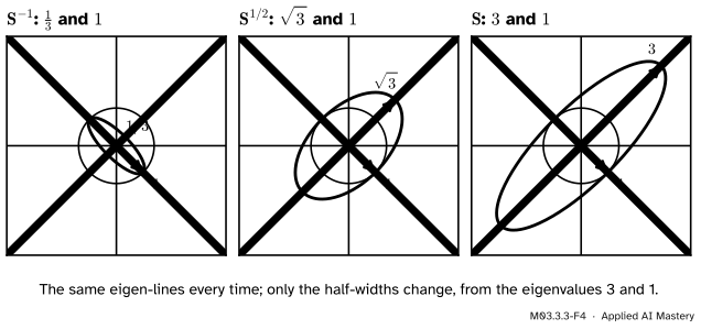
Inverse. If no eigenvalue is 0, let \(\mat{T} = {\sum_i \lambda_i^{-1}\mat{P}_i}\). Then \({\mat{S}\mat{T}} = {\sum_i \lambda_i\lambda_i^{-1}\mat{P}_i} = {\sum_i \mat{P}_i} = \mat{I}\), so \(\mat{T} = {\mat{S}^{-1}}\).
Square root. If no eigenvalue is negative, let \({\mat{S}^{1/2}} = {\sum_i \sqrt{\lambda_i}\,\mat{P}_i}\). Its square is \({\sum_i \lambda_i\mat{P}_i} = \mat{S}\), it is symmetric, and its eigenvalues \({\sqrt{\lambda_i}}\) are not negative. It is the only matrix with all three properties (Axler 7.39).
M03.3.3-F4
\({\mat{S}^{-1}}\), \({\mat{S}^{1/2}}\) and \(\mat{S}\) share the eigenvectors of \(\mat{S}\). Only the stretch on each line changes: \({\tfrac13}\), \({\sqrt{3}}\) and 3 along \(\vect{q}_1\), and \(1\) along \(\vect{q}_2\) in all three.
Keeping only the big pieces. If some eigenvalues are much larger than the rest, the pieces with small \(\abs{\lambda_i}\) change \(\mat{S}\) little, and dropping them leaves a matrix of lower rank that does almost the same job. For \(\mat{S}\), keeping only \({3\mat{P}_1}\) leaves an error of exactly \({1\,\mat{P}_2}\). Module M03.6 makes this precise for any matrix, through the singular value decomposition; for a covariance matrix it is the core of principal component analysis.
Worked example
Split \(\mat{S}\) and the 3 by 3 matrix \(\mat{S}_3\) into pieces, then find \({\mat{S}^{-1}}\), \(\mat{S}^5\) and \({\mat{S}^{1/2}}\).
On \(\vect{x} = {(2, 0)}\): \(\mat{P}_1\vect{x} = {(1, 1)}\) and \(\mat{P}_2\vect{x} = {(1, -1)}\), so \(\mat{S}\vect{x} = {3\,(1, 1) + (1, -1)} = {(4, 2)}\), as in the anchor figure.
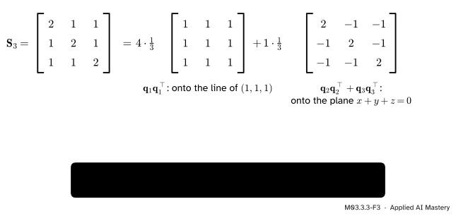
The 3 by 3 case.\(\mat{S}_3 = \begin{bmatrix} 2 & 1 & 1 \\ 1 & 2 & 1 \\ 1 & 1 & 2 \end{bmatrix}\) has eigenvalue 4 with \(\vect{q}_1 = {(1, 1, 1)/\sqrt{3}}\), and the repeated eigenvalue 1 on the plane \({x + y + z} = 0\) (last lesson). Every entry of \(\vect{q}_1\vect{q}_1\T\) is \({\tfrac{1}{\sqrt3} \cdot \tfrac{1}{\sqrt3}} = {\tfrac13}\). The two pieces for the eigenvalue 1 add up to \({\mat{P}_2 + \mat{P}_3} = {\mat{I} - \mat{P}_1}\), by the third fact of Step 3, whichever orthonormal pair is chosen in the plane.
M03.3.3-F3
\(\mat{S}_3\) as 4 times the projection onto a line plus 1 times the projection onto the plane perpendicular to it. The yellow box checks every entry.
Functions of \(\mat{S}\). Apply each function to 3 and 1 and keep the pieces:
Checks. \(\mat{S}\) times the first column of \({\mat{S}^{-1}}\) is \({\tfrac13(4 - 1,\; 2 - 2)} = {(1, 0)}\). The entries of \(\mat{S}^5\) are \({243/2 + 1/2} = 122\) and \({243/2 - 1/2} = 121\), as lesson M02.9.4 found the long way. And the top-left entry of the square of \({\mat{S}^{1/2}}\) is \({\tfrac14\big((\sqrt3 + 1)^2 + (\sqrt3 - 1)^2\big)} = {\tfrac14(4 + 2\sqrt3 + 4 - 2\sqrt3)} = 2\), while the top-right is \({\tfrac14 \cdot 2(\sqrt3 + 1)(\sqrt3 - 1)} = {\tfrac14 \cdot 2 \cdot 2} = 1\). Numerically, \(\mat{S}^{1/2} \approx \begin{bmatrix} 1.366 & 0.366 \\ 0.366 & 1.366 \end{bmatrix}\).
Code
From scratch: rebuild a symmetric matrix from its pieces, then apply any function through the eigenvalues.
import mathimport numpy as npdef pieces(S):"""Eigenvalues and the projection matrices q q^T of a symmetric matrix.""" lam, Q = np.linalg.eigh(S)return lam, [np.outer(Q[:, i], Q[:, i]) for i inrange(len(lam))]def apply_function(S, f):"""f(S) = sum of f(lambda_i) q_i q_i^T.""" lam, P = pieces(S)returnsum(f(l) * p for l, p inzip(lam, P))S = np.array([[2.0, 1.0], [1.0, 2.0]])S3 = np.array([[2.0, 1.0, 1.0], [1.0, 2.0, 1.0], [1.0, 1.0, 2.0]])lam, P = pieces(S)print("eigenvalues:", lam.round(10))print("pieces:\n", P[0].round(6), "\n", P[1].round(6))print("sum of lambda_i P_i:\n", sum(l * p for l, p inzip(lam, P)).round(10))print("S x by pieces:", sum(l * (p @ [2.0, 0.0]) for l, p inzip(lam, P)).round(10))
eigenvalues: [1. 3.]
pieces:
 [[ 0.5 -0.5]
 [-0.5  0.5]]
 [[0.5 0.5]
 [0.5 0.5]]
sum of lambda_i P_i:
 [[2. 1.]
 [1. 2.]]
S x by pieces: [4. 2.]
The order of eigh is ascending, so its first piece belongs to the eigenvalue 1. Now the three functions, each checked against an independent library route.
Last, the glimpse of low rank: keep only the biggest piece of a symmetric matrix and measure what is lost. The size of a matrix here is the square root of the sum of its squared entries, a measure that module M03.8 studies.
rng = np.random.default_rng(1)X = rng.normal(size=(200, 3)) @ np.array([[3.0, 0.0, 0.0], [1.0, 1.0, 0.0], [0.5, 0.2, 0.3]])C = np.cov(X, rowvar=False) # a 3 by 3 covariance matrixlam, P = pieces(C)keep_one = lam[-1] * P[-1] # the piece with the largest eigenvaluesize =lambda M: math.sqrt((M **2).sum())print("eigenvalues of C:", lam.round(3))print("share of the size lost by keeping one piece:", round(size(C - keep_one) / size(C), 3))
eigenvalues of C: [0.077 0.809 8.837]
share of the size lost by keeping one piece: 0.092
One piece out of three keeps almost all of this covariance matrix. With the eigenvalues numbered from the largest, \({\lambda_1 \ge \lambda_2 \ge \lambda_3}\), the error is the size of the two dropped pieces, which is \({\sqrt{\lambda_2^2 + \lambda_3^2}}\), because the pieces are perpendicular to one another.
Explore
The spectral ellipse in lesson M03.3.2 has a Pieces switch. Turn it on and turn the angle slider: the chosen vector is projected onto each eigen-line, each shadow is stretched by its eigenvalue, and the two stretched shadows add up to the image. Make one eigenvalue negative and watch its piece point backwards.
Pitfalls
M03.3.3-F5
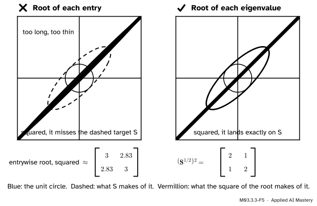
Wrong beside right. Taking the square root of each entry of \(\mat{S}\) gives a matrix whose square is not \(\mat{S}\). Taking the square root of each eigenvalue does.
“np.sqrt(S) is the square root of the matrix, and S ** 2 is its square.”
Both work entry by entry. np.sqrt(S) has entries \({\sqrt2}\) and 1, and its square is about \(\begin{bmatrix} 3 & 2.83 \\ 2.83 & 3 \end{bmatrix}\), not \(\mat{S}\). S ** 2 has entries 4 and 1, while \({\mat{S}\mat{S}} = \begin{bmatrix} 5 & 4 \\ 4 & 5 \end{bmatrix}\). Use S @ S, np.linalg.matrix_power, scipy.linalg.sqrtm, or the pieces.
“Any eigenvector will do in the piece \({\lambda\,\vect{v}\vect{v}\T}\).”
Only a unit vector gives a projection. With \(\vect{v} = {(1, 1)}\), \({\vect{v}\vect{v}\T} = \begin{bmatrix} 1 & 1 \\ 1 & 1 \end{bmatrix}\) is twice \(\mat{P}_1\), and \({3\vect{v}\vect{v}\T + \ldots}\) overshoots. Divide by \({\vect{v}\T\vect{v}}\), or normalise first.
“Every symmetric matrix has a square root.”
Not a real symmetric one. The square of a real symmetric matrix \(\mat{R}\) has the eigenvalues \({\mu_i^2 \ge 0}\), where the \(\mu_i\) are the real eigenvalues of \(\mat{R}\). The running saddle has the eigenvalue \({-1}\), so no real symmetric matrix squares to it. The square root of this lesson needs every eigenvalue to be at least 0: the positive semidefinite matrices of module M03.4, which include every covariance matrix.
Check yourself
Recall
1. Write a symmetric matrix as a sum of pieces, and say what each piece is.
Show answer
\(\mat{S} = {\sum_i \lambda_i\vect{q}_i\vect{q}_i\T}\). Each \(\vect{q}_i\vect{q}_i\T\) is the projection onto the line of the unit eigenvector \(\vect{q}_i\), scaled by its eigenvalue.
2. Why is \(\vect{q}\vect{q}\T\vect{x}\) the projection of \(\vect{x}\) onto the line of a unit vector \(\vect{q}\)?
Show answer
\({\vect{q}\vect{q}\T\vect{x}} = {\vect{q}(\vect{q}\T\vect{x})} = {(\vect{q} \cdot \vect{x})\vect{q}}\), the formula for the projection onto a unit vector.
3. What are \(\mat{P}_1\mat{P}_1\), \(\mat{P}_1\mat{P}_2\) and \({\mat{P}_1 + \mat{P}_2}\) for the pieces of a symmetric 2 by 2 matrix?
Show answer
\(\mat{P}_1\), the zero matrix, and \(\mat{I}\).
4. How do you compute \({\mat{S}^{-1}}\) from the pieces, and when does it exist?
Show answer
\({\mat{S}^{-1}} = {\sum_i \lambda_i^{-1}\mat{P}_i}\), which exists when no eigenvalue is 0.
5. Which matrix is \({\mat{S}^{1/2}}\) for the running \(\mat{S}\), roughly?
1.★ Write the running saddle \(\begin{bmatrix} 1 & 2 \\ 2 & 1 \end{bmatrix}\) as a sum of two pieces, and use them to compute its effect on \({(2, 0)}\).
Show solution
Its eigenvalues are 3 and \({-1}\) with the same eigenvectors as \(\mat{S}\), so the saddle is \({3\mat{P}_1 - \mat{P}_2}\). Check: \({\tfrac32\begin{bmatrix} 1 & 1 \\ 1 & 1 \end{bmatrix} - \tfrac12\begin{bmatrix} 1 & -1 \\ -1 & 1 \end{bmatrix}}\) has diagonal entries \({\tfrac32 - \tfrac12} = 1\) and off-diagonal entries \({\tfrac32 + \tfrac12} = 2\). On \({(2, 0)}\): \({3\,(1, 1) - (1, -1)} = {(2, 4)}\), which is the saddle’s first column times 2.
2.★★ Find the symmetric square root, with no negative eigenvalues, of \(\mat{M} = \begin{bmatrix} 5 & 4 \\ 4 & 5 \end{bmatrix}\).
Show solution
\(\mat{M}\) sends \({(1, 1)}\) to \({(9, 9)}\) and \({(1, -1)}\) to \({(1, -1)}\), so it has the eigenvalues 9 and 1 with the pieces \(\mat{P}_1\) and \(\mat{P}_2\) of \(\mat{S}\). Its square root is \({\sqrt9\,\mat{P}_1 + \sqrt1\,\mat{P}_2} = {3\mat{P}_1 + \mat{P}_2} = \mat{S}\). Indeed \({\mat{S}\mat{S}} = \begin{bmatrix} 4 + 1 & 2 + 2 \\ 2 + 2 & 1 + 4 \end{bmatrix} = \mat{M}\).
3.★★★ Prove that \({\mat{S}^k} = {\sum_i \lambda_i^k\mat{P}_i}\) for every whole number \({k \ge 1}\), using only the three facts of Step 3.
Show solution
By induction on \(k\). For \(k = 1\) it is the spectral decomposition. Suppose it holds for \(k\). Then
Every term with \({i \neq j}\) is zero, because \({\mat{P}_i\mat{P}_j} = \mat{0}\). The terms with \(i = j\) are \({\lambda_i^{k+1}\mat{P}_i\mat{P}_i} = {\lambda_i^{k+1}\mat{P}_i}\). So \({\mat{S}^{k+1}} = {\sum_i \lambda_i^{k+1}\mat{P}_i}\), which is the claim for \({k + 1}\).
Summary card
A symmetric matrix is a weighted sum of projections onto perpendicular lines.
M03.3.3-F1
Project, scale, add.
Pieces.\(\mat{S} = {\sum_i \lambda_i\vect{q}_i\vect{q}_i\T}\), with \({\vect{q}\vect{q}\T\vect{x}} = {(\vect{q} \cdot \vect{x})\vect{q}}\).
Low rank. Drop the pieces with small \(\abs{\lambda_i}\) (module M03.6).
Sources and next steps
Sources. Each was opened and checked against this lesson on 15 November 2026.
Gilbert Strang, Symmetric matrices and positive definiteness, MIT OpenCourseWare 18.06SC, lecture 25 summary, part “Projection onto eigenvectors”: writing \({\mat{Q}\mat{\Lambda}\mat{Q}\T}\) column by row gives \({\lambda_1\vect{q}_1\vect{q}_1\T + \cdots + \lambda_n\vect{q}_n\vect{q}_n\T}\), and each \({\vect{q}_k\vect{q}_k\T}\) is a projection matrix, so every symmetric matrix is a combination of perpendicular projection matrices.
Sheldon Axler, Linear Algebra Done Right, 4th edition (open access). Result 7.39: every positive operator has exactly one positive square root; notation 7.40 writes it \({\sqrt{T}}\). (For a self-adjoint operator, Axler’s “positive” means that no eigenvalue is negative.)
Marc Peter Deisenroth, A. Aldo Faisal and Cheng Soon Ong, Mathematics for Machine Learning (free PDF), Section 4.4, eigendecomposition and diagonalisation: a symmetric matrix is \({\mat{P}\mat{D}\mat{P}\T}\) with orthonormal eigenvectors, and powers are taken through the diagonal factor.
SciPy reference, scipy.linalg.sqrtm: the matrix square root, used here only as an independent check.