Read a dense layer, multi-head attention scores and a low-rank weight matrix as contractions with named axes: every reshape, transpose, einsum and softmax with its shape, worked by hand on two tokens and two heads, then in NumPy.
M03.10.4L2 Intermediate25 minIn review (what this means)
The maths and code on this page are checked by automated tests on every change, but an independent reader has not signed it off yet. Spot a mistake or a confusing step? Tell us.
Write a dense layer on a batch as y_bj = x_bi w_ji + c_j, and give the shape of every array in it.
Trace multi-head attention scores step by step (reshape, transpose, einsum, scale, softmax), stating each shape.
Explain the 1/sqrt(d_h) scale and why the softmax runs along the key axis.
Count the parameters and the multiply-adds of a weight matrix written as two thin factors, and relate it to low-rank approximation.
The question
A transformer layer receives a batch of 2 sentences of 4 tokens, each token described by 8 numbers, and computes attention with 2 heads. Between the input and the attention weights the numbers pass through five arrays, laid out in four different ways. One wrong axis and the layer still runs, quietly mixing heads or tokens. Can you name every axis of every array on the way?
From the last lesson
1. In bhtd,bhsd->bhts, which letter is summed, and what is the output shape when \(b = 2\), \(h = 2\), \(t = s = 4\), \(d = 4\)?
Show answer
\(d\), the only letter missing from the output. The output keeps \(b, h, t, s\): shape (2, 2, 4, 4).
2. What does np.einsum("ij,jh", A, B) return, and why?
Show answer
The transpose of \(\mat{A}\mat{B}\). In implicit mode the output letters are sorted alphabetically, so the output is hi, not ih.
Intuition
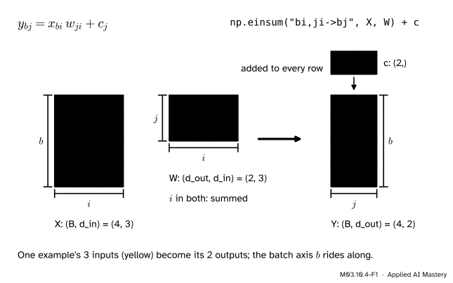
A dense layer sends each example’s vector of \(d_{\text{in}}\) numbers through the same weight matrix and adds the same bias. On a batch, that is one contraction: the batch axis rides along, the input axis is summed, and the output axis is new.
M03.10.4-F1
A dense layer on a batch of 4 examples. The letter \(i\) is in both \(\mat{X}\) and \(\mat{W}\) and not in the output, so it is summed; \(b\) is kept on its own, so each example is handled separately.
Everything else in this lesson is the same game with more axes. Attention adds an axis for the head and a second axis for the token, and a low-rank layer splits one weight matrix into two thin ones. Each step is a reshape, a transpose or a contraction from the last three lessons.
Build it up
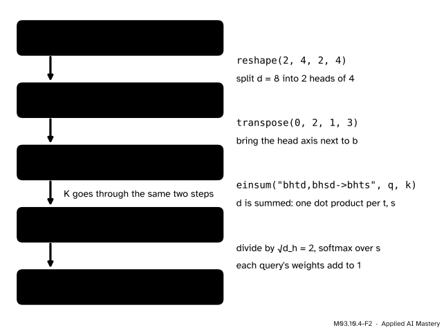
Multi-head attention scores, with the example sizes \(B = 2\), \(T = 4\), \(d = 8\) and \(h = 2\) heads of \(d_h = d / h = 4\).
Step 1. Queries and keys. Two dense layers turn the input of shape (B, T, d) into queries \(\mat{Q}\) and keys \(\mat{K}\) of the same shape (DL05.1 builds them). Here they are simply given.
Step 2. Split the embedding into heads. Reshape (B, T, d) to (B, T, h, dh). This only splits the last axis into two neighbouring axes, so the reading order is kept: embedding entry \(e\) goes to head \(\lfloor e / d_h \rfloor\), position \(e \bmod d_h\). A reshape is right here.
Step 3. Bring the head axis forward. Transpose with the tuple \((0, 2, 1, 3)\) to (B, h, T, dh). Now each head is a separate (T, dh) matrix, like a batch.
Step 4. Scores. Contract queries with keys over the head entry: np.einsum("bhtd,bhsd->bhts", q, k). The letter \(d\) is summed; here it runs over the \(d_h\) entries of one head, not over the full width \(d\). The letter \(t\) indexes the query token and \(s\) the key token, so the result has shape (B, h, T, T).
Step 5. Scale and normalise. Divide by \(\sqrt{d_h}\) and take the softmax along \(s\), so that each query’s weights over the keys are positive and add to 1.
M03.10.4-F2
Multi-head attention scores, one shape per step. Only the reshape and the transpose touch the layout; the einsum does the arithmetic.
Step
Shape
Here
Q, K
(B, T, d)
(2, 4, 8)
split heads
(B, T, h, dh)
(2, 4, 2, 4)
transpose
(B, h, T, dh)
(2, 2, 4, 4)
scores, weights
(B, h, T, T)
(2, 2, 4, 4)
The formal statement
NoteDefinitions: dense layer, attention scores and weights
A dense layer with weight \(\mat{W}\) of shape \((d_{\text{out}}, d_{\text{in}})\) and bias \(\vect{c}\) of length \(d_{\text{out}}\) maps a batch \(\mat{X}\) of shape \((B, d_{\text{in}})\) to \(y_{bj} = x_{bi}\, w_{ji} + c_j\).
For queries and keys split into heads, \(q_{bhtd}\) and \(k_{bhsd}\), the scaled scores and the attention weights are
The dense layer in matrix form. Since \((\mat{W}\T)_{ij} = w_{ji}\), the sum \(x_{bi} w_{ji} = x_{bi} (\mat{W}\T)_{ij} = (\mat{X}\mat{W}\T)_{bj}\). So \(\mat{Y} = \mat{X}\mat{W}\T + \vect{c}\), with \(\vect{c}\) broadcast to every row. This is exactly the layout of PyTorch’s nn.Linear, which stores its weight as (out_features, in_features).
The weights of each query add to 1. Fix \(b, h, t\). The denominator does not depend on \(s\), so
The two sums are the same sum with the dummy renamed. Every weight is positive, because \(e^{z} > 0\).
Why divide by \(\sqrt{d_h}\). Suppose the entries of \(\vect{q}\) and \(\vect{k}\) are independent, with mean 0 and variance 1. Then each product \(q_d k_d\) has mean \({\E[q_d]\,\E[k_d]} = 0\) and variance \({\E[q_d^2]\,\E[k_d^2]} = 1\), and the \(d_h\) products are independent, so
A raw score is typically \(\sqrt{d_h}\) in size; for \(d_h = 64\) that is 8. Scores that large push the softmax into regions where its gradients are extremely small (Vaswani et al.), with nearly all the weight on one key. Dividing by \(\sqrt{d_h}\) brings the variance back to 1.
The cost of the scores. The einsum loops over \(b, h, t, s, d\): \(B h T^2 d_h\) multiply-adds. Since \(h d_h = d\), that is \(B T^2 d\), the same as a single head of the full width.
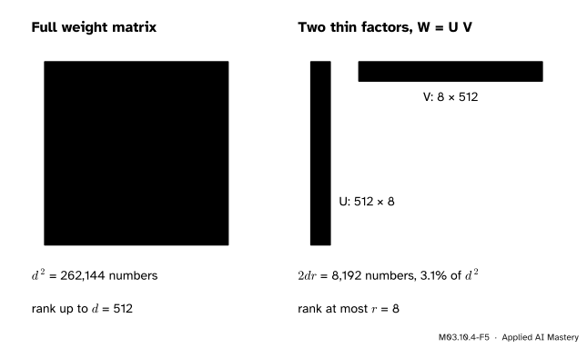
A weight matrix of low rank. Write a \(d \times d\) weight as \(\mat{W} = \mat{U}\mat{V}\) with \(\mat{U}\) of shape \((d, r)\) and \(\mat{V}\) of shape \((r, d)\), \(r\) much smaller than \(d\). In index notation \(w_{ji} = u_{jk} v_{ki}\), and the layer becomes
It stores \(2dr\) numbers instead of \(d^2\). Every column of \(\mat{U}\mat{V}\) is \(\mat{U}\) times a column of \(\mat{V}\), so it lies in the column space of \(\mat{U}\) and the rank is at most \(r\). Computed in the cheap order, first \(z_{bk} = x_{bi} v_{ki}\) and then \(y_{bj} = z_{bk} u_{jk}\), it costs \(2Bdr\) multiply-adds instead of \(Bd^2\). To approximate a given \(\mat{W}\) by such a product, the best choice in the Frobenius and spectral norms is the truncated SVD of M03.6.1.
M03.10.4-F5
A \(512 \times 512\) weight against two thin factors of rank 8: 3.1% of the numbers.
Frontier note: low-rank updates in fine-tuning
LoRA (Hu et al., 2021) keeps a large pre-trained weight \(\mat{W}_0\) frozen and trains only a low-rank change \(\Delta\mat{W} = \mat{B}\mat{A}\), with \(\mat{B}\) of shape \((d, r)\) and \(\mat{A}\) of shape \((r, k)\) and \(r\) much smaller than \(d\) and \(k\): the factorisation above applied to the update. Parameter-efficient tuning is the subject of A02.5.
Worked example
Two tokens, two heads, by hand. Take \(B = 1\), \(T = 2\), \(d = 4\), \(h = 2\), \(d_h = 2\). The queries of the two tokens are \((1, 1, 2, 0)\) and \((1, -1, 0, 1)\); the keys are \((1, 1, 0, 1)\) and \((1, -1, 1, 0)\).
Split. Head 0 takes the first two entries of every token, head 1 the last two. So head 0 has queries \((1, 1)\), \((1, -1)\) and keys \((1, 1)\), \((1, -1)\); head 1 has queries \((2, 0)\), \((0, 1)\) and keys \((0, 1)\), \((1, 0)\).
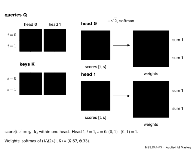
Scores. Each score is a dot product within one head, rows \(t\) and columns \(s\):
Scale and softmax. Divide by \(\sqrt{2}\). For two scores \(z_1, z_2\) the softmax weight of the first is \({1 / (1 + e^{-(z_1 - z_2)})}\). Row 0 of head 0 has difference \(2/\sqrt{2} = 1.414\), giving \({1 / (1 + e^{-1.414})} = 0.804\) and \(0.196\). Row 1 of head 1 has difference \(1/\sqrt{2} = 0.707\), giving \(0.670\) and \(0.330\).
M03.10.4-F3
The worked example as a trace. Each head has its own score matrix; each row of weights adds to 1, and the yellow cell is the key that query attends to most.
Token 0 in head 0 attends mostly to key 0 (0.80); in head 1 it attends mostly to key 1 (0.80). Two heads, two different patterns from the same tokens: that is the point of having heads.
Code
The dense layer three ways, and the shapes asserted.
scores, head 0: [[2.0, 0.0], [0.0, 2.0]]  head 1: [[0.0, 2.0], [1.0, 0.0]]
weights, head 0: [[0.804, 0.196], [0.196, 0.804]]  head 1: [[0.196, 0.804], [0.67, 0.33]]
shapes: (2, 2, 4, 4)  matmul agrees: True  rows sum to 1: True
The variance argument, by simulation, and the low-rank layer with its counts and its rank.
dh =64q_s, k_s = rng.normal(size=(20_000, dh)), rng.normal(size=(20_000, dh))dots = np.einsum("nd,nd->n", q_s, k_s)print("variance of raw scores:", dots.var().round(1), " after dividing by sqrt(dh):", (dots / np.sqrt(dh)).var().round(3))d, r, Bn =512, 8, 32U, V = rng.normal(size=(d, r)), rng.normal(size=(r, d))Xn = rng.normal(size=(Bn, d))print("parameters:", d * d, "against", 2* d * r, f"({2* r / d:.1%})", " rank of UV:", np.linalg.matrix_rank(U @ V))y_full = np.einsum("bi,ji->bj", Xn, U @ V)y_low = np.einsum("bi,ki,jk->bj", Xn, V, U, optimize=True)print("same output:", np.allclose(y_full, y_low), " multiply-adds:", Bn * d * d, "against", 2* Bn * d * r)
variance of raw scores: 64.3   after dividing by sqrt(dh): 1.004
parameters: 262144 against 8192 (3.1%)   rank of UV: 8
same output: True   multiply-adds: 8388608 against 262144
The simulated variance is close to 64, as derived, and close to 1 after scaling; both are random, so the check allows a small tolerance.
Explore
The einsum explorer of M03.10.3 has the attention string as a preset, bhtd,bhsd->bhts. Set the sizes of this lesson and watch the cost: doubling \(t\) and \(s\) together multiplies it by four, which is why long contexts are expensive. Then type bi,ji->bj, the dense layer.
Pitfalls
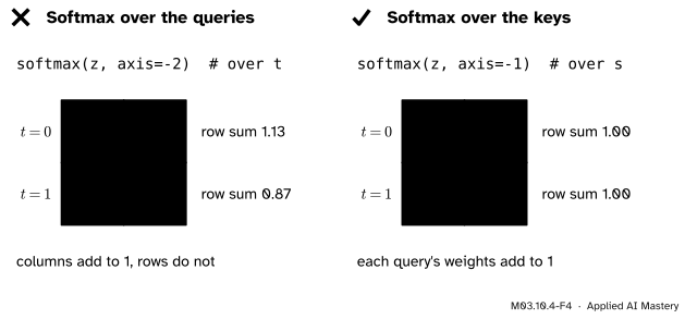
M03.10.4-F4
Wrong beside right, on head 1 of the worked example. Only the softmax over the key axis \(s\) gives each query a set of weights that adds to 1.
“The softmax axis does not matter much.”
It decides what the weights mean. Over \(s\) (the last axis) each query distributes one unit of attention among the keys. Over \(t\) the columns add to 1 instead. Head 0 of the worked example has a symmetric score matrix, so both axes give the same numbers there and the mistake hides; test with scores that are not symmetric.
“Reshape straight to (B, h, T, dh) and skip the transpose.”
The reshape keeps the reading order, which runs token by token. Reshaping the worked queries straight to (1, 2, 2, 2) makes “head 0” the two halves of token 0, \((1, 1)\) and \((2, 0)\), instead of the first halves of both tokens. Split the last axis first, then transpose (lesson M03.10.1).
“X @ W is the dense layer.”
With \(\mat{W}\) stored as \((d_{\text{out}}, d_{\text{in}})\) the layer is X @ W.T. When \(d_{\text{in}} \neq d_{\text{out}}\), X @ W raises a shape error; when they are equal it runs and is wrong. Writing np.einsum("bi,ji->bj", X, W) names the summed axis and removes the doubt.
Check yourself
Recall
1. Write a dense layer on a batch in index notation, with the weight stored as \((d_{\text{out}}, d_{\text{in}})\).
Show answer
\({y_{bj} = x_{bi} w_{ji} + c_j}\), or np.einsum("bi,ji->bj", X, W) + c, which is X @ W.T + c.
2. Which two operations turn queries of shape (B, T, d) into shape (B, h, T, dh), in which order?
Show answer
First reshape to (B, T, h, dh), splitting the last axis; then transpose with \((0, 2, 1, 3)\).
3. Along which axis does the attention softmax run, and what does it guarantee?
Show answer
Along \(s\), the key axis (the last one). Each query’s weights are positive and add to 1.
4. Why are the scores divided by \(\sqrt{d_h}\)?
Show answer
With independent entries of mean 0 and variance 1, a dot product of length \(d_h\) has variance \(d_h\). Dividing by \(\sqrt{d_h}\) brings it back to 1, so the softmax is not pushed to extremes.
5. How many numbers does a \(d \times d\) weight store, and how many does \(\mat{U}\mat{V}\) with inner size \(r\) store?
Show answer
\(d^2\) against \(2dr\). For \(d = 512\) and \(r = 8\), 262,144 against 8,192.
Exercises
1.★ A dense layer maps width 768 to width 3072. How many parameters does it have, counting the bias? What is its subscript string and output shape on an input of shape (32, 128, 768)?
Show solution
Weights \({768 \cdot 3072} = 2{,}359{,}296\), plus 3,072 biases: 2,362,368. On a batch of sequences the string is bti,ji->btj (both \(b\) and \(t\) ride along) and the output has shape (32, 128, 3072).
2.★★ Attention with \(B = 8\), \(T = 128\), \(d = 512\) and \(h = 8\) heads. Give \(d_h\), the shape after each step, and the multiply-adds of the score einsum. Compare with one head of width 512.
Show solution
\(d_h = 512 / 8 = 64\). Shapes: (8, 128, 512), then (8, 128, 8, 64), then (8, 8, 128, 64), then scores and weights (8, 8, 128, 128). The einsum loops over \(b, h, t, s, d\):
One head of width 512 costs \({8 \cdot 128 \cdot 128 \cdot 512}\), the same number, because \(h \cdot d_h = d\).
3.★★★ Prove that \(\mat{U}\mat{V}\), with \(\mat{U}\) of shape \((d, r)\) and \(\mat{V}\) of shape \((r, d)\), has rank at most \(r\). Then, for \(d = 4096\) and \(r = 16\), give the share of parameters kept and the multiply-adds per example of the cheap order against the full matrix.
Show solution
Column \(i\) of \(\mat{U}\mat{V}\) is \(\mat{U}\) times column \(i\) of \(\mat{V}\), a combination of the \(r\) columns of \(\mat{U}\). So every column lies in the column space of \(\mat{U}\), whose dimension is at most \(r\), and the rank, the dimension of the column space of \(\mat{U}\mat{V}\), is at most \(r\).
Parameters: \(2dr = 131{,}072\) against \(d^2 = 16{,}777{,}216\), a share of \(2r/d = 1/128\), about 0.78%. Per example the cheap order costs \(dr + rd = 131{,}072\) multiply-adds against \(d^2\): the same ratio.
Summary card
A layer is a contraction with named axes: keep the batch, sum the input, create the output.
M03.10.4-F1
\(y_{bj} = x_{bi}\, w_{ji} + c_j\).
Dense:np.einsum("bi,ji->bj", X, W) + c = X @ W.T + c.
Scores:bhtd,bhsd->bhts, divide by \(\sqrt{d_h}\), softmax over \(s\); cost \(B T^2 d\).
Low rank:\(w_{ji} = u_{jk} v_{ki}\): \(2dr\) numbers instead of \(d^2\), rank at most \(r\).
Sources and next steps
Sources. Each was opened and checked against this lesson on 15 November 2026.
Ashish Vaswani and others, Attention Is All You Need (2017). Section 3.2.1, equation (1): attention as the softmax of \(\mat{Q}\mat{K}\T / \sqrt{d_k}\); the reason for the scale, with the footnote that independent components of mean 0 and variance 1 give a dot product of variance \(d_k\). Section 3.2.2: \(h = 8\) heads with \(d_k = d_{\text{model}}/h = 64\), at a total cost similar to single-head attention of full width.
PyTorch reference, torch.nn.Linear: the layer computes \(y = x A\T + b\) with weight of shape (out_features, in_features), on inputs of shape (*, in_features).
Edward J. Hu and others, LoRA: Low-Rank Adaptation of Large Language Models (2021), section 4.1: the update of a weight \(\mat{W}_0\) of shape \(d \times k\) written as \(\mat{B}\mat{A}\) with \(\mat{B}\) of shape \(d \times r\), \(\mat{A}\) of shape \(r \times k\) and \(r\) much smaller than \(d\) and \(k\).
NumPy reference, numpy.einsum, for the subscript strings and the optimize argument used in the code.
Next. DL05.1, Self-attention from scratch, adds the query, key and value projections and the weighted sum of values; A02.5, Parameter-efficient tuning, trains low-rank updates. This lesson closes the course; its other modules are listed on the course page.