Principal component analysis finds the directions in which a cloud of data spreads most. Centre the data, form the covariance matrix, and its eigenvectors are those directions; derive why, and why the same line makes the perpendicular gaps as small as possible.
M03.6.3L2 Intermediate25 minIn review (what this means)
The maths and code on this page are checked by automated tests on every change, but an independent reader has not signed it off yet. Spot a mistake or a confusing step? Tell us.
Centre a data matrix and form its covariance matrix C = X_c-transpose X_c / (n - 1).
Derive that the variance of the data along a unit direction u is u-transpose C u, and that its largest value is the top eigenvalue, reached along the top eigenvector.
Compute the principal directions, their variances and the explained-variance ratios of a small data set by hand and with numpy.linalg.eigh.
Prove with Pythagoras that the direction of largest variance is also the line through the mean with the smallest sum of squared perpendicular gaps.
The question
A data set with fifty measurements per item cannot be drawn: we see in two dimensions, three at a push. Before clustering it, plotting it or feeding it to a model, we would like to know which directions in that fifty-dimensional space the data actually uses. Which single direction shows the most of a cloud of points, and how do we find it?
From the last lesson
1. How many numbers does it take to store \(k\) layers of an \(m \times n\) picture?
Show answer
\(k(m + n + 1)\), against \(mn\) for the picture itself.
2. A truncation keeps 99% of the energy. What is its relative error?
Show answer
The square root of the share dropped: \(\sqrt{0.01} = 10\%\).
Intuition
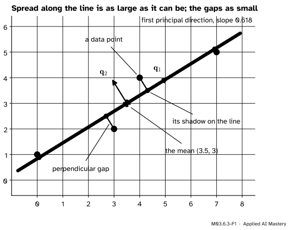
Take the running four points \((0, 1)\), \((3, 2)\), \((4, 4)\) and \((7, 5)\). Draw a line through their mean and drop each point straight onto it, at a right angle. The dropped points, the shadows, are spread out along the line. Turn the line, and the spread of the shadows changes.
M03.6.3-F1
The first principal direction of the four points. Along this line the shadows (vermillion) spread out the most, and the perpendicular gaps (purple) are the smallest.
The direction in which the shadows spread most is the first principal direction. It is the one direction that keeps the most of what distinguishes the points from one another. Principal component analysis, PCA, finds it, then the best direction perpendicular to it, and so on. The same line also hugs the points as closely as possible, measured at right angles; that is the promise made in the pitfalls of M02.10.4.
Build it up
Step 1. Centre. Subtract the mean from every point. The mean of the four points is \((3.5, 3)\), and the centred points are the rows of
Each column of \(\mat{X}_c\) now adds up to zero. Spread is measured from the centre of the cloud, so this is the right place to stand.
Step 2. The shadow of one point. For a unit vector \(\vect{u}\) and a centred point \(\vect{x}_i\), the shadow is \({(\vect{u} \cdot \vect{x}_i)\,\vect{u}}\), and its signed position along the line is the number \(\vect{u} \cdot \vect{x}_i\), called the score of the point. The four scores are the entries of \(\mat{X}_c\vect{u}\). They add up to zero, because each column of \(\mat{X}_c\) does.
Step 3. The variance of the scores. Their mean is zero, so their sample variance is the sum of their squares divided by \(n - 1\):
The middle step writes the squared length as \({(\mat{X}_c\vect{u})\T(\mat{X}_c\vect{u})}\) and uses \({(\mat{X}_c\vect{u})\T} = {\vect{u}\T\mat{X}_c\T}\). The matrix \(\mat{C} = {\mat{X}_c\T\mat{X}_c/(n - 1)}\) is the covariance matrix of the data (M06.10.2): its diagonal holds the variances of the features, and off the diagonal sit their covariances.
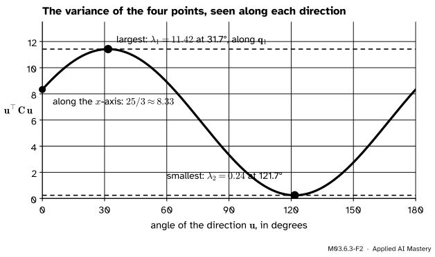
Step 4. Turn the direction. With \(\vect{u} = {(\cos\theta, \sin\theta)}\), the variance \(\vect{u}\T\mat{C}\vect{u}\) is a smooth function of the angle. Plot it and read off the best angle.
M03.6.3-F2
The variance of the four points seen along each direction. The highest and lowest points of the curve are exactly the two eigenvalues of \(\mat{C}\), and they sit \(90°\) apart.
The formal statement
Result 1: the direction of largest variance. Let \(\mat{C}\) have eigenvalues \(\lambda_1 \ge \lambda_2 \ge \cdots \ge \lambda_d\) and orthonormal eigenvectors \(\vect{q}_1, \dots, \vect{q}_d\), as the spectral theorem promises for a symmetric matrix (M03.3.2). Then over all unit vectors \(\vect{u}\), the variance \(\vect{u}\T\mat{C}\vect{u}\) is largest, equal to \(\cparam{\lambda_1}\), at \(\vect{u} = \cparam{\vect{q}_1}\).
Why. This is the Rayleigh quotient of M03.3.4. Write \(\vect{u}\) in the eigenbasis, \(\vect{u} = {c_1\vect{q}_1 + \cdots + c_d\vect{q}_d}\), with \({c_1^2 + \cdots + c_d^2} = 1\) because \(\vect{u}\) is a unit vector. Then \(\mat{C}\vect{u} = \sum_i c_i\lambda_i\vect{q}_i\) and
with equality when \(c_1 = \pm 1\) and the rest are zero, that is at \(\vect{u} = \pm\vect{q}_1\).
Result 2: the later directions. Among unit vectors perpendicular to \(\vect{q}_1\), so with \(c_1 = 0\), the same line of algebra gives at most \(\lambda_2\), reached at \(\vect{q}_2\). Going on, the \(j\)-th principal direction is \(\vect{q}_j\), perpendicular to all the earlier ones, and the variance along it is \(\lambda_j\).
Result 3: explained variance. The total variance is the sum of the variances of the features, the trace of \(\mat{C}\), which equals the sum of its eigenvalues (M03.1.3). So the directions share it out exactly, and the explained-variance ratio of direction \(j\) is
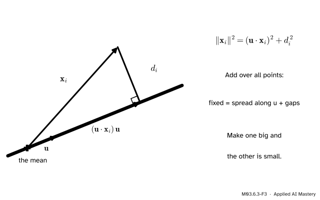
Result 4: largest spread, smallest gaps. For a centred point \(\vect{x}_i\) and a unit \(\vect{u}\), the shadow and the perpendicular gap \(d_i\) are the two sides of a right-angled triangle whose long side is \(\vect{x}_i\).
M03.6.3-F3
Pythagoras for one point. Its squared distance from the mean is fixed; turning the line only moves it between the shadow and the gap.
By Pythagoras, \({\norm{\vect{x}_i}^2} = {(\vect{u} \cdot \vect{x}_i)^2 + d_i^2}\). Add over the points and use Step 3:
The left side does not depend on \(\vect{u}\). So the \(\vect{u}\) that makes the variance largest makes the sum of squared perpendicular gaps smallest: the first principal direction is the best fitting line through the mean, measured at right angles. The smallest sum of gaps is \({(n - 1)}\) times the variance left over.
Go deeper: why the best line passes through the mean
Let a line pass through a point \(\vect{p}\) in the direction \(\vect{u}\), and let \(\mat{G}\) be the matrix that removes the part along \(\vect{u}\), so the gap of a data point \(\vect{y}_i\) is \({\mat{G}(\vect{y}_i - \vect{p})}\). Write \(\vect{m}\) for the mean and split \(\vect{y}_i - \vect{p} = {(\vect{y}_i - \vect{m}) + (\vect{m} - \vect{p})}\). Expanding the squares,
where \(\vect{g} = {\mat{G}(\vect{m} - \vect{p})}\). The last sum is zero, because the deviations from the mean add up to zero. The middle term is never negative and vanishes when the line passes through \(\vect{m}\). So for any direction, moving the line to pass through the mean can only shrink the gaps.
Worked example
The running four points, by hand. From \(\mat{X}_c\) above, the scatter matrix is
since \({12.25 + 0.25 + 0.25 + 12.25} = 25\), \({7 + 0.5 + 0.5 + 7} = 15\) and \({4 + 1 + 1 + 4} = 10\). With \(n - 1 = 3\), \(\mat{C}\) is a third of it. The scatter matrix is easier to work with; its eigenvectors are those of \(\mat{C}\) and its eigenvalues are three times as big.
M03.6.3-F4
From four points to their first principal direction, in five steps.
Eigenvalues. The characteristic polynomial is \(\lambda^2 - 35\lambda + {(250 - 225)} = \lambda^2 - 35\lambda + 25\). Since \(35^2 - 4 \cdot 25 = 1125 = 225 \cdot 5\), the roots are
Variances. Dividing by 3, the variances along the two principal directions are about \(11.42\) and \(0.24\). The total variance is \({(25 + 10)/3} \approx 11.67\), the sum of the variances of \(x\) (\(8.33\)) and \(y\) (\(3.33\)). The first direction explains \({\lambda_1/(\lambda_1 + \lambda_2)} = \tfrac12 + \tfrac{3\sqrt5}{14} \approx 97.9\%\) of it.
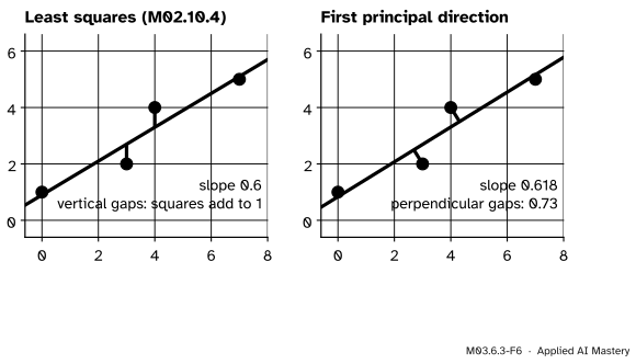
The promise of M02.10.4. The least-squares line through these points has slope \(0.6\); the first principal direction has slope \(0.618\). Both pass through the mean, but they answer different questions.
M03.6.3-F6
Two best lines. Least squares makes the vertical gaps small; the first principal direction makes the perpendicular gaps small.
The perpendicular gaps of the principal line have squares adding to the smaller eigenvalue of the scatter matrix, \({(35 - 15\sqrt5)/2} \approx 0.729\), by Result 4. The least-squares line has smaller vertical gaps (1 against about 1.01) but larger perpendicular ones (about 0.735).
Code
From scratch: centre, form \(\mat{C}\), take its eigenvectors with numpy.linalg.eigh and sort them by size. eigh returns the eigenvalues in ascending order, so we reverse.
import numpy as npdef pca_eigh(X):"""Principal directions (as columns), their variances and the explained-variance ratios.""" X = np.asarray(X, dtype=float) Xc = X - X.mean(axis=0) C = Xc.T @ Xc / (len(X) -1) variances, directions = np.linalg.eigh(C) # ascending order order = np.argsort(variances)[::-1] variances, directions = variances[order], directions[:, order]return directions, variances, variances / variances.sum(), Cpoints = np.array([[0.0, 1.0], [3.0, 2.0], [4.0, 4.0], [7.0, 5.0]])Q, lam, ratio, C = pca_eigh(points)print("C =\n", C.round(4))print("variances:", lam.round(4), " ratios:", ratio.round(4))print("slope of the first direction:", round(Q[1, 0] / Q[0, 0], 4))
C =
 [[8.3333 5.    ]
 [5.     3.3333]]
variances: [11.4235  0.2432]   ratios: [0.9792 0.0208]
slope of the first direction: 0.618
Now check Results 1 and 4 on many directions: the variance never beats \(\lambda_1\), and variance plus gaps is always the same total.
Xc = points - points.mean(axis=0)angles = np.linspace(0, np.pi, 3601)best, total_ok =-np.inf, Truefor a in angles: u = np.array([np.cos(a), np.sin(a)]) variance = u @ C @ u gaps = np.sum((Xc - np.outer(Xc @ u, u)) **2) # squared perpendicular gaps total_ok &= np.isclose(3* variance + gaps, np.sum(Xc **2)) best =max(best, variance)print("largest variance found:", round(best, 4), " lambda_1:", round(lam[0], 4))print("variance and gaps always add up to the same total:", total_ok)u_ls = np.array([1.0, 0.6]) / np.hypot(1.0, 0.6) # direction of the least-squares lineprint("perpendicular gaps, principal line:", round(np.sum((Xc - np.outer(Xc @ Q[:, 0], Q[:, 0])) **2), 4)," least-squares line:", round(np.sum((Xc - np.outer(Xc @ u_ls, u_ls)) **2), 4))
largest variance found: 11.4235   lambda_1: 11.4235
variance and gaps always add up to the same total: True
perpendicular gaps, principal line: 0.7295   least-squares line: 0.7353
The search over 3,601 directions never beats \(\lambda_1\), and comes within \(10^{-5}\) of it.
Explore
The module’s interactive, the rank slider, is in lesson M03.6.2. Its bars are the singular values of a picture; the next lesson shows that the variances of PCA are squared singular values too, divided by \(n - 1\), so the same picture of kept and dropped bars describes a PCA.
Pitfalls
M03.6.3-F5
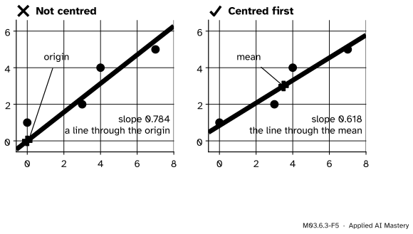
Wrong beside right. Without centring, the top eigenvector of \({\mat{X}\T\mat{X}}\) describes where the cloud sits as seen from the origin, not how it spreads.
“I can skip centring; the eigenvectors will sort it out.”
Without centring, \(\vect{u}\T\mat{X}\T\mat{X}\vect{u}\) counts the distance of the points from the origin, not from their mean. For the four points, the top eigenvector of \(\mat{X}\T\mat{X} = \begin{bmatrix} 74 & 57 \\ 57 & 46 \end{bmatrix}\) has slope about \(0.784\), pulled towards the direction of the mean, \((3.5, 3)\), which has slope \(0.857\). The spread of the cloud has slope \(0.618\).
“The first principal direction is the regression line.”
Regression predicts \(y\) from \(x\), so it measures errors in \(y\) only, vertically. PCA treats the features alike and measures at right angles. On the four points the slopes are \(0.6\) and \(0.618\); on noisier data they can differ a lot. Use regression to predict a target, PCA to describe the shape of the data.
“Dividing by \(n\) instead of \(n - 1\) gives different components.”
M06.10 and some textbooks divide by \(n\). That multiplies every eigenvalue of \(\mat{C}\) by the same factor, so the directions and the explained-variance ratios do not change; only the variances themselves differ, by the factor \((n - 1)/n\).
Check yourself
Recall
1. Why must the data be centred before PCA?
Show answer
Variance is spread about the mean. Without centring, \(\vect{u}\T\mat{X}\T\mat{X}\vect{u}\) measures distances from the origin, and the top direction points towards the mean instead of along the spread.
2. What is the variance of the data along a unit direction \(\vect{u}\)?
Show answer
\(\vect{u}\T\mat{C}\vect{u}\), with \(\mat{C} = {\mat{X}_c\T\mat{X}_c/(n - 1)}\).
3. Which direction makes that variance largest, and what is the largest value?
Show answer
The eigenvector \(\vect{q}_1\) of \(\mat{C}\) for the largest eigenvalue, and the value is \(\lambda_1\).
4. What is the explained-variance ratio of the \(j\)-th principal direction?
Show answer
\({\lambda_j/\operatorname{tr}(\mat{C})}\), its eigenvalue divided by the sum of all the eigenvalues.
5. Why does the direction of largest variance also give the smallest perpendicular gaps?
Show answer
By Pythagoras, each point’s squared distance from the mean is its squared score plus its squared gap. The total of the squared distances is fixed, so making the scores spread most makes the gaps smallest.
Exercises
1.★ Data have covariance matrix \(\mat{C} = \begin{bmatrix} 4 & 0 \\ 0 & 1 \end{bmatrix}\). What are the principal directions and the explained-variance ratios?
Show solution
\(\mat{C}\) is diagonal, so its eigenvectors are \((1, 0)\) and \((0, 1)\) with eigenvalues 4 and 1. The first principal direction is the \(x\)-axis, with ratio \(4/5 = 80\%\), and the second is the \(y\)-axis, with \(20\%\). When the features are uncorrelated, PCA simply ranks them by variance.
2.★★ Find the principal directions, their variances and the sum of the squared perpendicular gaps to the first one, for the points \((2, 1)\), \((1, 2)\), \((-2, -1)\) and \((-1, -2)\).
Show solution
The mean is \((0, 0)\), so the points are already centred. The scatter matrix is
since \({4 + 1 + 4 + 1} = 10\) and \({2 + 2 + 2 + 2} = 8\). Its eigenvectors are \({(1, 1)/\sqrt2}\) with eigenvalue 18 and \({(1, -1)/\sqrt2}\) with eigenvalue 2. Dividing by \(n - 1 = 3\), the variances are 6 and \(2/3\), and the first direction explains \(18/20 = 90\%\). By Result 4 the squared perpendicular gaps to the line \(y = x\) add up to 2: each point is \(1/\sqrt2\) from it, and \({4 \times \tfrac12} = 2\).
3.★★★ Show that projecting the centred data onto the span of the first \(k\) principal directions keeps a variance of \({\lambda_1 + \cdots + \lambda_k}\), that is \({\sum_i \norm{\text{projection of }\vect{x}_i}^2/(n - 1)} = {\lambda_1 + \cdots + \lambda_k}\).
Show solution
The directions \(\vect{q}_1, \dots, \vect{q}_k\) are orthonormal, so the projection of \(\vect{x}_i\) onto their span is \({\sum_{j \le k} (\vect{q}_j \cdot \vect{x}_i)\,\vect{q}_j}\), and its squared length is the sum of the squared coefficients, \({\sum_{j \le k} (\vect{q}_j \cdot \vect{x}_i)^2}\). Sum over the points, divide by \(n - 1\) and swap the two sums:
using Step 3 for each \(\vect{q}_j\) and \(\mat{C}\vect{q}_j = \lambda_j\vect{q}_j\) with \(\vect{q}_j\T\vect{q}_j = 1\). With \(k = d\) this is all of \(\operatorname{tr}(\mat{C})\).
Summary card
The principal directions are the eigenvectors of the covariance matrix.
M03.6.3-F1
Most spread, smallest gaps.
Centre and form.\(\mat{C} = {\mat{X}_c\T\mat{X}_c/(n - 1)}\).
Variance along \(\vect{u}\).\(\vect{u}\T\mat{C}\vect{u}\), largest (\(\lambda_1\)) at \(\vect{q}_1\).
Pythagoras. Largest variance along a line means smallest perpendicular gaps to it.
Sources and next steps
Sources. Each was opened and checked against this lesson on 15 November 2026.
David Austin, Understanding Linear Algebra, Principal component analysis. The variance of demeaned data in the direction of a unit vector \(\vect{u}\) is the quadratic form \({\vect{u} \cdot (C\vect{u})}\), the principal components are the eigenvectors of the covariance matrix in order of decreasing eigenvalue, and projecting onto the first \(n\) of them keeps the sum of the first \(n\) eigenvalues. Austin stores the points as columns and divides by \(N\), not \(N - 1\).
Marc Deisenroth, Aldo Faisal and Cheng Soon Ong, Mathematics for Machine Learning, Chapter 10. Equation (10.1) defines the data covariance matrix of centred data; Section 10.2 derives PCA as maximising the variance of the projected data, and Section 10.3 as minimising the reconstruction error, the two views of Result 4.
NumPy, numpy.linalg.eigh: for a symmetric matrix it returns the eigenvalues in ascending order and the normalised eigenvectors as columns.
Next.M03.6.4 PCA by SVD, in practice gets the same directions without ever forming \(\mat{C}\), and applies them to real measurements.